I built an interactive Shiny application that uses simulated annealing to solve the famous traveling salesman problem. You can play around with it to create and solve your own tours at the bottom of this post, and the code is available on GitHub.

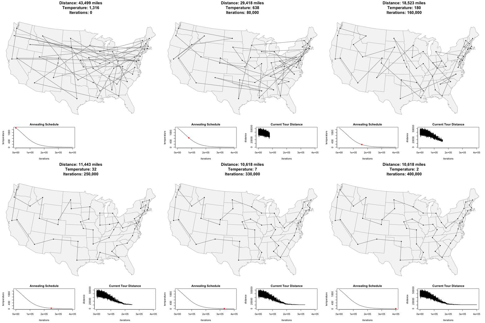
Here’s an animation of the annealing process finding the shortest path through the 48 state capitals of the contiguous United States:

How does the simulated annealing process work?

We start by picking an arbitrary initial tour from the set of all valid tours. From that initial tour we “move around” and check random neighboring tours to see how good they are. There are so many valid tours—(47! / 2), to be exact—that we won’t be able to test every possible solution. But a well-designed annealing process eventually reaches a solution that, if it is not the global optimum, is at least good enough. Here’s a step-by-step guide:

1. Start with a random tour through the selected cities. Note that it’s probably a very inefficient tour!
2. Pick a new candidate tour at random from all neighbors of the existing tour. Via Professor Joe Chang, one way to pick a neighboring tour “is to choose two cities on the tour randomly, and then reverse the portion of the tour that lies between them.” This candidate tour might be better or worse compared to the existing tour, i.e. shorter or longer.
3. If the candidate tour is better than the existing tour, accept it as the new tour.
4. If the candidate tour is worse than the existing tour, still maybe accept it, according to some probability. The probability of accepting an inferior tour is a function of how much longer the candidate is compared to the current tour, and the temperature of the annealing process. A higher temperature makes you more likely to accept an inferior tour.
5. Go back to step 2 and repeat many times, lowering the temperature a bit at each iteration, until you get to a low temperature and arrive at your (hopefully global, possibly local) minimum. If you’re not sufficiently satisfied with the result, try the process again, perhaps with a different temperature cooling schedule.

The key to the simulated annealing method is in step 4: even if we’re considering a tour that is worse than the tour we already have, we still sometimes accept the worse tour temporarily, because it might be the stepping stone that gets us out of a local minimum and ultimately closer to the global minimum. The temperature is usually pretty high at the beginning of the annealing process, so that initially we’ll accept more tours, even the bad ones. Over time, though, we lower the temperature until we’re only accepting new tours that improve upon our solution.

If you look at the bottom 2 graphs of the earlier USA animation, you can see that at the beginning the “Current Tour Distance” jumps all over the place while the temperature is high. As we turn the temperature down, we accept fewer longer tours and eventually we converge on the globally optimal tour.

What’s the point?

That’s all well and good, but why do we need the annealing step at all? Why not do the same process with 0 temperature, i.e. accept the new tour if and only if it’s better than the existing tour? It turns out if we follow this naive “hill climbing” strategy, we’re far more likely to get stuck in a local minimum. Histograms of the results for 1,000 trials of the traveling salesman through the state capitals show that simulated annealing fares significantly better than hill climbing:

Simulated annealing doesn’t guarantee that we’ll reach the global optimum every time, but it does produce significantly better solutions than the naive hill climbing method. The results via simulated annealing have a mean of 10,690 miles with standard deviation of 60 miles, whereas the naive method has mean 11,200 miles and standard deviation 240 miles.

And so, while you might not think that Nikolay Chernyshevsky or Chief Wiggum would be the best people to offer an intuition behind simulated annealing, it turns out that they, along with cliche-spewers everywhere, understand the simple truth behind simulated annealing: sometimes things really do have to get worse before they can get better.

Make your own tour with the interactive Shiny app

Here’s the Shiny app that lets you pick up to 30 cities on the map, set some parameters of the annealing schedule, then run the actual simulated annealing process (or just click ‘solve’ if you’re lazy). Give it a shot below! Bonus points if you recognize where the default list of cities comes from…

The app is hosted at ShinyApps.io, but if you want to run the app on your local machine, it’s very easy, all you need to do is paste the following into your R console:

1
2
3

install.packages(c("shiny", "maps", "geosphere"), repos="https://cran.rstudio.com/")
library(shiny)
runGitHub("shiny-salesman", "toddwschneider")

Code on GitHub

The full code is available on GitHub

Around the World in 80,000 Miles

Here’s another animated gif using a bunch of world capitals. The “solution” here is almost certainly not the global optimum, but it’s still fun to watch!