In particular, although the dataset does not explicitly indicate when high-demand “surge” pricing was in effect, I used the available fields to reverse engineer the historical surge pricing map based on a robust regression model. More to come about the methodology, along with challenges and caveats. All code used in this post is available on GitHub. As I write this in March 2020, the dataset includes 129 million trips from November 1, 2018 through December 31, 2019. It is scheduled to update quarterly in the future.
You can play around with the map below to see estimated surge pricing multipliers by time and neighborhood. I’ve highlighted some notable events with elevated pickup activity and/or surge pricing, for example at the conclusion of The Rolling Stones concert at Soldier Field on June 25, 2019, when fares were 3x more expensive than usual.
Click here to view map in full screen or on a mobile device
In addition to estimated surge multipliers, the map shows modified z-scores, which represent pickup activity in an area compared to the median for that time of day and day of week. Positive z-scores mean more pickups than normal. For example, the area near Soldier Field saw 154 pickups at midnight after the Stones concert, while a median Wednesday midnight sees 9 pickups with a median absolute deviation of 2.5. Those numbers produce a large modified z-score of 39, meaning way more pickups than normal. (The “modified” part in modified z-score refers to the use of the median and median absolute deviation instead of the mean and standard deviation, which reduces the impact of outliers.)
It’s often interesting to compare the map of surge multipliers to the map of modified z-scores, since Uber and Lyft both state that surge pricing goes into effect when there are more riders than drivers in an area. The dataset does not explicitly tell us how many drivers are available at any given moment, but it seems like a reasonable assumption that sudden demand spikes and higher-than-normal pickup activity would often coincide with rider demand outstripping driver supply.
The conclusion of the aforementioned Rolling Stones No Filter Tour show on June 25, 2019 appears to have been one of the most severe surge pricing events in the dataset. I isolated trips that began near Soldier Field on the Near South Side, then compared surge prices to pickup counts at each 15-minute interval. The graph shows that surge prices and pickup activity both started to increase around 11:30 PM. Peak surge occurred between midnight and 12:30 AM, which coincided with the largest number of pickups.
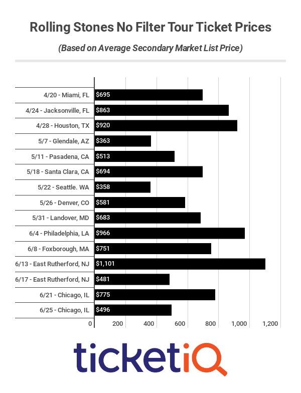
I couldn’t find the exact time they played each song on the setlist, but I’d guess that the encore of “Gimme Shelter” and “(I Can’t Get No) Satisfaction” began just before midnight, and the 11:30 PM pickups peak represents people who tried to beat the traffic and skipped the encore, while the larger 12:15 AM pickups peak includes the folks who stuck around until the very end. The 11:30 PM departures paid a significantly lower average surge of 1.7x compared to 3.2x for the 12:15 AM crowd, though with ticket prices already averaging $500, I’m not so sure that would have been a major consideration.
The June 25 show was the Stones’s second Soldier Field date; they kicked off their 2019 North American tour a few nights earlier on June 21, and the ride-hailing activity patterns look pretty much the same. The first show saw a bit more pickup activity than the second show, but a slightly lower peak surge rate of 2.9x.
The next-most severe Soldier Field surge pricing events belonged to another major concert tour, though one that perhaps catered to a different audience than the Stones. K-pop supergroup BTS played two Soldier Field dates on May 11 and 12, 2019 as part of their Love Yourself: Speak Yourself world tour. The average post-concert surge prices on night one and night two reached as high as 2.5x.
Soldier Field is home for the NFL’s Chicago Bears, but strangely enough, Bears games do not show much evidence of surge pricing compared to The Rolling Stones and BTS concerts, even though Bears games do exhibit similar demand spikes at the conclusion of games.
Here’s a representative graph of ride-hail activity immediately following a Bears home game. (Apologies to Bears fans, but as an Eagles fan, I must confess that I look back fondly on the Double Doink.)
None of the Bears home games in the dataset appear to have produced major spikes in surge pricing. The biggest post-game pickup spikes were a pair of 2019 regular season Thursday night games against the Packers and Cowboys, both of which show similar patterns to the Eagles game: a large spike in post-game pickups, but only a small corresponding increase in surge prices. The biggest post-game surge I could find occurred after a December 2019 Sunday night game against the Chiefs, but the peak surge of 1.4x was still significantly lower than the rates seen at the Stones and BTS concerts.
One possibility is that drivers are somehow more “aware” of Bears games than concerts, so they’re more likely to make themselves available in the vicinity of Soldier Field after Bears games than concerts, and the excess supply of cars prevents surge pricing from kicking in. The dataset does not provide any information on how many drivers were available in an area at a given time, so this would be a difficult idea to test, but there might be a creative way to get at it. We also don’t know how many people tried to hail a ride but then for whatever reason didn’t. For example, though pickups peaked at around 300 per 15 minutes after both the Stones concert and the Eagles game, maybe there were more people trying to hail rides after the concert.
There are plenty of theories we could come up with to explain the Bears/Stones discrepancy, but if I had to guess, the most likely explanation is a major caveat that runs throughout this entire post: it seems like most of the major surge events citywide occurred in Q2 2019—specifically between March 29 and June 30—so much so that it makes me wonder if there is an error or other hidden bias in the dataset. If there is a Q2 2019 bias, then regardless of whether it’s a data error, a change in surge pricing algorithms, or something else, the May/June concerts might have more severe surge pricing than the September–January Bears games due to a hidden variable, not an underlying truth that concerts produce higher surge prices than football games.
The United Center tells a similar story. Located on the Near West Side, it hosts the NBA’s Bulls and NHL’s Blackhawks, a number of major concerts from Ariana Grande to Travis Scott, and other one-off events like UFC 238 and a Michelle Obama book reading. Much like at Soldier Field, the highest surge pricing rates seem to come at the conclusion of concerts, but again I’m concerned about the Q2 2019 bias.
Neither the Bulls nor the Blackhawks made their respective leagues’ playoffs in 2019, so there weren’t many NBA/NHL games that took place in April/May/June. The few games that took place in April 2019 did show some significant surge pricing compared to games that took place in other months. For example, the Bulls hosted the Knicks on both April 9, 2019, and November 12, 2019. Both games were on Tuesday nights, both saw similar numbers of post-game pickups, yet only the April 9 game had significant surge pricing.
The two biggest United Center concerts, as measured by spikes in total pickups, belonged to Mumford & Sons on March 29, 2019, and Travis Scott on December 6, 2018. Both concerts had similar-sized spikes in pickups, but post-Mumford & Sons surge pricing reached 2.7x, while post-Travis Scott peaked at a more mild 1.4x. Again though, March 29 was the beginning of the 3-month period of elevated surge pricing citywide, so it’s possible that some hidden bias accounts for the elevated surge.
Of course I’ve cherry-picked these examples to fit a narrative, but you can head over to GitHub to see surge pricing graphs for every date on the United Center events calendar.
Concerts and sporting events are obvious candidates for surge pricing because they involve large groups of people trying to leave the same place at the same time, which could easily overwhelm the supply of available drivers. But there are also examples of more geographically diffuse surge pricing events, often coinciding with holidays or inclement weather.
One of the biggest citywide surge incidents occurred on the morning of Monday, April 29, 2019. It rained heavily that morning, and by 6:00 AM, surge prices reached 2x across most of the city’s North Side. As rush hour peaked around 8:00 AM, riders stretching from Lake View to Hyde Park were paying 2-3 times their normal fares. By 9:30 AM, the surge had died down and fares were back to normal.
If you look at the map of z-scores during the April 29 surge, demand was somewhat elevated compared to a typical Monday morning, but not dramatically so, and certainly not as severely as after a big concert. Again, we don’t know exactly how many drivers were available that morning. It’s possible that the bad weather initially made drivers less inclined to work, which led to high surge prices to incentivize more drivers to become available.
Other events that caused elevated demand across the entire city include New Year’s Eve, Super Bowl LIII, Saint Patrick’s Day Parade, Pride Parade, and the late night hours of Thanksgiving Eve—the unfortunately-titled “Blackout Wednesday.” Of that list, the 2019 Pride Parade looks to have generated the highest surge pricing, but again it occurred during the Q2 2019 era of generally elevated surge pricing, so it could be an artifact of that as opposed to something more meaningful.
The unexplained Q2 2019 discrepancy makes it difficult to say anything meaningful about general surge pricing trends, but it seems like there are some patterns when you look at certain regions by time of week. For example, on the North Side—a generally affluent area with high rider demand on weekday mornings as people commute into Central Chicago—weekday surge prices tend to be highest in the morning. The magnitude is more severe during the Q2 2019 period, but the 8:00 AM–9:00 AM hour appears to be the most expensive throughout the year.
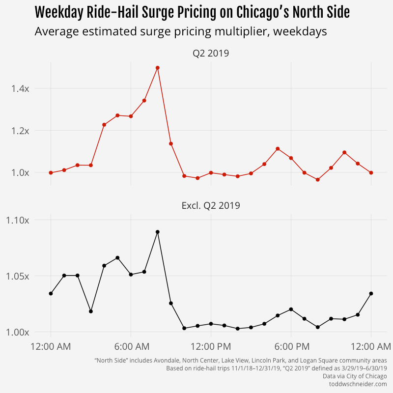
The North Side also sees a lot of pickups on weekday afternoons, but surge prices are significantly lower during afternoons compared to mornings. One possibility is that there are more cars available in the afternoon. The weekday afternoon route from Central Chicago to the North Side is very common, so maybe that produces a surplus of available drivers on the North Side, which in turn drives down fares for afternoon riders getting picked up on the North Side. I didn’t dig into that idea any deeper, but it could make for an interesting follow up.
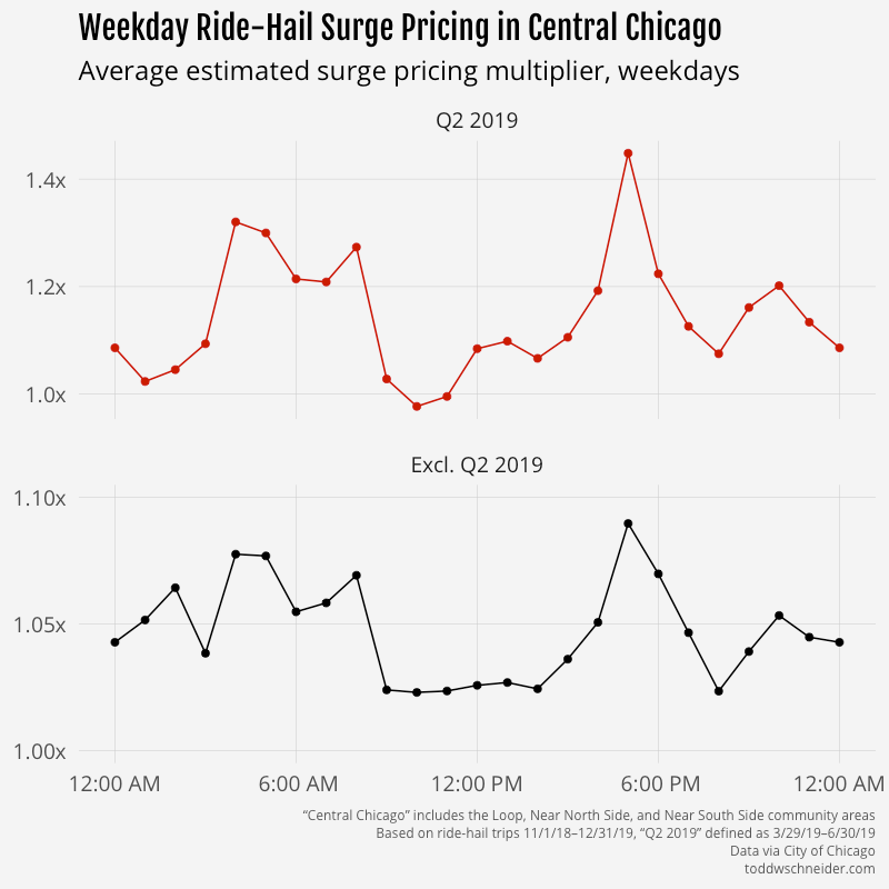
In Central Chicago, where demand is highest on weekday afternoons as people head home after work, surge prices are highest during afternoon rush hour.
And on the West Side, where demand is generally highest on weekend evenings, surge prices are highest in the late night weekend hours.
The dataset does not explicitly tell us when surge pricing was in effect, but it provides fields that allow us to estimate: trip distance, travel time, and fare amount. Uber and Lyft do not say exactly how they determine fares, but they both indicate on their websites [Uber, Lyft] that fares are based on a combination of distance and time.
I first calibrated a robust regression model of fare as a linear combination of distance and time, then estimated the surge multiplier for each trip as its actual fare divided by the baseline predicted fare. For example, if a 4-mile, 15-minute trip had an actual fare of $15, but the baseline model predicted it should have been a $10 fare, then the estimated surge multiplier for that trip is 1.5x.
After I estimated multipliers for each trip, I bucketed by pickup census tract and timestamp rounded to 15 minutes, and took the simple unweighted average of all surge multipliers within each bucket. In some cases, when tract-level info wasn’t available, I aggregated by the larger community area geographies.
The naive temptation for the baseline model might be to fit a linear regression via ordinary least squares, for example using R’s lm() function. However, in this case I don’t think that’s the right way to fit the baseline model, because an OLS linear regression will find parameters that make the average predicted fare equal to the average actual fare. But we don’t want to fit our baseline model against all fares, rather we want to fit it against some notion of “typical” fares, excluding surge and other pricing abnormalities like discounts. This presents a circular logic problem:
Robust regression methods are designed to address this circular problem. I chose the rlm() function from R’s MASS package with the “MM” option, which uses an iterative process to find coefficients of a linear model, determine outliers based on those coefficients, downweight or even remove the outliers entirely, find new coefficients, and repeat until some convergence criteria are met.
I found that the coefficients from the robust model implied base fares were 12% lower than implied by the OLS model during the Q2 2019 period, and 3% lower in other periods. The robust coefficients also aligned more closely with the indicative rate cards posted on Uber and Lyft’s websites, which provides some reassurance that the robust methodology is a reasonable estimate of non-surge fares.
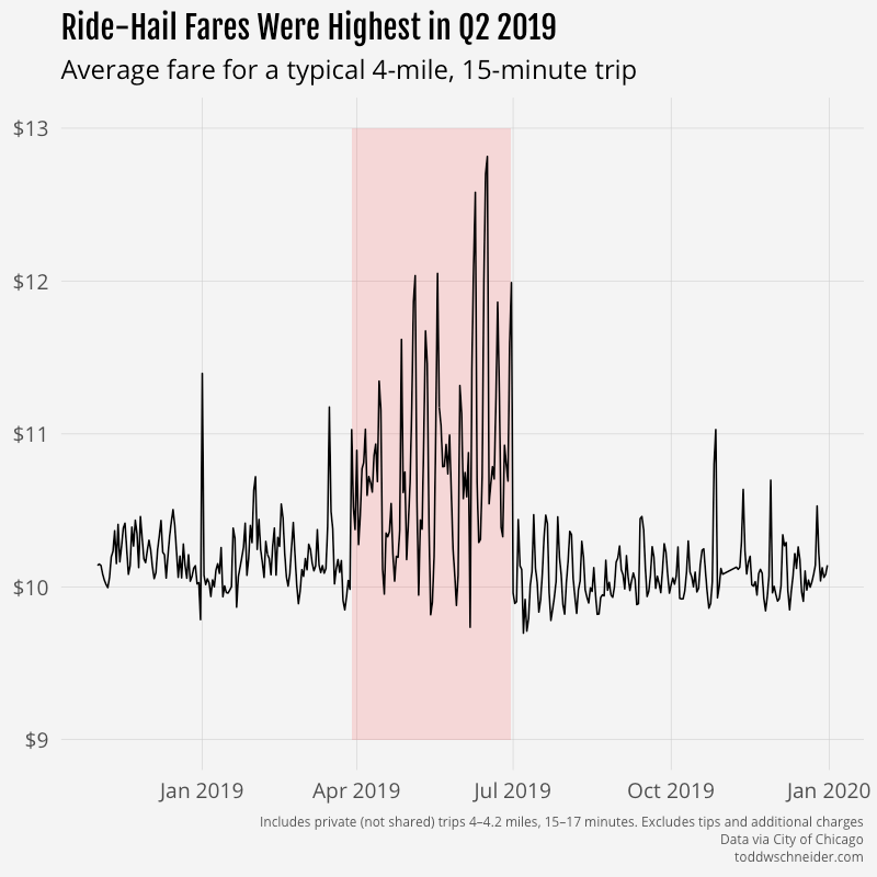
The period from March 29, 2019 through June 30, 2019 appears to contain a disproportionate number of major surge pricing events compared to the rest of the dataset.
My first thought was that maybe Uber and/or Lyft changed their base fare rates during that time period, so I split the dataset into three pricing regimes—before, during, and after Q2—and calibrated separate robust regression models for each regime. Here are the resulting model coefficients:
Time period | Intercept | Fare per mile | Fare per minute |
---|---|---|---|
Before 3/29/19 | $1.81 | $0.82 | $0.28 |
3/19/19–6/30/19 | $2.13 | $0.82 | $0.27 |
After 6/30/19 | $1.87 | $0.82 | $0.27 |
The coefficients on distance and time were nearly identical in all 3 regimes: 82 cents per mile, plus 27–28 cents per minute. The intercept for the Q2 regime was around 30 cents higher than for the other periods, which amounts to a bit over 2% of the average $13 fare.
The fact that the robust regression coefficients from Q2 are not drastically different than the periods before and after argues, but does not prove, that base fare rates were not different during the Q2 period. My best guess is that one or both of Uber and Lyft made some changes that resulted in more aggressive surge pricing in Q2 2019, but then reverted those changes on or around July 1. I’m still wary though that there could be a data reporting error; it will be interesting to see what happens as more trip data is published in the future.
There are other possibilities to consider, e.g. maybe there’s a spring seasonal effect, perhaps due to elevated rider demand following the long, cold winter. Unfortunately it’s hard to know much about time-of-year seasonality since there’s only one year of data available. The particularly abrupt apparent surge pricing decrease on July 1 argues against a seasonal effect, and to me suggests something like an algorithm change or a data reporting error.
There was a story from May 2019 about drivers in Washington, D.C. attempting to manipulate surge pricing algorithms by simultaneously turning off their apps to create the appearance of a driver shortage. I have no particular insight into the strategy’s existence, effectiveness, or presence in Chicago, but I suppose it’s possible that the story led to Uber and Lyft changing their surge pricing algorithms.
I’m not sure how we could confirm an algorithm change, as Uber and Lyft don’t seem likely to reveal their secret sauce anytime soon. For what it’s worth, March 29, 2019—the first day of elevated surge estimates—was also Lyft’s first day as a publicly-traded company. Uber’s IPO followed a few weeks later on May 10. I suppose it’s as least possible that they increased their surge rates around then in an effort to demonstrate revenue growth to Wall Street, but it strikes me as unlikely given all of the coordination required.
Surge pricing is one of many factors beyond time and distance that can impact a single trip’s fare. The dataset does not provide explicit info about these additional factors, so I made some oversimplifications and assumptions and that are worth noting.
Uber and Lyft both offer an array of vehicle classes—standard, luxury, SUV, etc.—each of which has a different base rate. The dataset does not include the vehicle class for each trip, so the model assumes that all fares have the same base rate, which we know isn’t true. The robust regression model will tend to fit the baseline against the most “typical” fares, which might include only the standard vehicle tier. If that’s the case, and, say, trips from the central business district are more likely to request luxury vehicles, then it could appear that the CBD has higher “surge prices”, when in reality the higher prices are driven at least in part by corporate riders’ tendency to request more luxurious vehicles.
Surge pricing makes fares more expensive than normal, but Uber and Lyft sometimes offer promotional discounts that make fares cheaper than normal. I’m hopeful that the robust regression methodology handles discounts roughly correctly by identifying them as outliers and downweighting them, but there’s no easy way to confirm. There have been some reports that both companies are trying to cut back on discounts, which could make it appear that surge pricing is increasing over time, even though the underlying reality is a decrease in discounts as opposed to an increase in surge pricing.
Uber and Lyft both provide upfront prices based on expected time and distance, which in turn are presumably based on routing algorithms that take into account factors like traffic and weather. If a trip’s actual time and distance end up differing from the expectations baked into the upfront price, my methodology might incorrectly interpret the fare as either a surge or a discount. Both companies say that they revise upfront fares for trips that materially deviate from expectation, so hopefully that mitigates some of this concern.
We could try to control for some of these hidden factors in the baseline model, for example by adding explanatory variables based on geography and time of week, but without any actual data that isolates the effects of surge pricing, discounts, vehicle class, and upfront pricing, I’d worry that the results would end up as a mishmash of all of them, which is essentially what the existing baseline model already is.
The City of Chicago takes some measures to protect rider, driver, and company privacy in the data. I very much support the privacy measures overall, but they do make it somewhat harder to estimate surge pricing. In particular, the dataset has the following privacy-oriented limitations:
Fares are rounded to the nearest multiple of $2.50. This reduces the precision on surge multiplier estimates, especially for smaller fares. For example, if a trip’s baseline expected fare is $4.00, but a surge of 1.5x is in effect so the actual fare is $6.00, that surge will never show up in the data because both $4.00 and $6.00 will round to $5.00. I attempted to control for this by excluding shorter trips when calculating average surge multipliers. Specifically, I restricted to fares that were at least 1.5 miles or 8 minutes. One nice reassurance is that my baseline model coefficients happen to align closely with the standard vehicle rates posted on Uber and Lyft’s websites.
Pickup and drop off timestamps are rounded to 15-minute intervals. If we’re looking at trips in an area between 12:00:00 PM and 12:14:59 PM, we won’t know which ones were at 12:00, 12:01, 12:02, etc. If surge pricing went into effect for just 2 minutes, the surge trips would get averaged in with trips from the other 13 minutes of the interval, resulting in a smoothed-out average surge multiplier. Additionally, the timestamps refer only to the time of pickup, but it might be relevant to know the timestamp when each rider submitted their ride request, as I’d imagine that’s a trigger for surge pricing algorithms.
Pickup and drop off geographies are imprecise, and sometimes redacted. Surge pricing can go into effect in very localized regions, as small as a few city blocks. But the Chicago dataset only provides pickup and drop off locations by census tract. Census tracts vary in size, but are almost always larger than a few city blocks, so if a surge goes into effect for a subregion of a tract, the tract-level aggregate will be smoothed-out. Additionally, census tracts are deliberately dropped in some cases where there are not enough pickups or drop offs over a 15-minute window. In such cases, locations are aggregated up to the community area level, which further reduces the precision of surge pricing estimates. Census tract-level data is available for about 75% of the trips in the dataset, the other 25% use community areas.
There are more general caveats beyond the potential hidden factors and privacy measures described above. Some trip records contain obvious junk data, e.g. a $1,000 fare for a 3-minute, 1-mile trip. I applied some heuristics to remove rows where I thought the data was an error, see GitHub for the exact logic.
The dataset does not provide info on which ride-hail company provided each trip, so there’s no obvious way to tell if Uber and Lyft have significantly different surge pricing behavior. As of March 2020 there are three companies registered to do business in Chicago: Uber, Lyft, and Via. A third party estimates their market shares as of November 2019 as 72% Uber, 27% Lyft, and 1% Via, which is not too far off from the known market shares in New York. (Of note, the New York dataset does include the company associated with each trip, but NYC does not provide fare info, so there’s no way to estimate surge pricing in NYC.)
In addition to the fare amount for each trip, the dataset also includes tips and “additional charges”, which cover taxes, fees, and tolls. I made the assumption that surge multipliers affect only the fare component, which seems consistent with the data, though I doubt the results would change much if I had used [fare + additional charges] as the dependent variable instead of fare only. Chicago added a new ride-hail tax in early 2020, which is not yet reflected in the data, but it will be interesting to see what happens as the dataset grows.
Shared rides present another challenge, because it’s not as clear how to establish a baseline fare. A more inconvenient route for a shared trip will increase both the time and distance, but it might make the fare cheaper since the rider might need an incentive to accept the longer route. About a third of shared trip requests don’t get matched, which is another important factor in determining the fare. I calibrated robust regressions for share-requested fares using time, distance, and whether the trip was matched, but it might make more sense to use “expected time/distance if following the most direct route” instead of actuals. I would want to do more research and investigation before feeling more confident about shared trip pricing. Making matters more confusing, it seems like there was a change in the way shared trip distances are reported starting in November 2019, when the average shared trip distance increased dramatically.
For the purposes of this post, I excluded trips with share requests when estimating surge multipliers, but I included trips with share requests when measuring rider demand, e.g. modified z-scores and pickup counts in the various graphs.
About 20% of trips in the dataset include a share request. Of those, about 68% get pooled into a shared trip, with the other 32% going unmatched. It seems like shared trips have become less popular over time; the months toward the beginning of the dataset have a higher percentage of share requests (~27%) and a higher match rate (~72%), but as of Q4 2019, only 15% of trips include a share request, with 60% of share requests get matched. See the shared trips section of the ride-hailing dashboard for the latest data.
There’s a lot of interesting work that could be done comparing Chicago’s public taxi and ride-hail datasets. As of December 2019, baseline private ride-hail trips are cheaper than taxis, and it looks like the “breakeven” surge is around 1.2x, meaning thax ride-hail trips are cheaper than taxis as long as the surge rate is 1.2x or lower. If you take tips into account, the breakeven is closer to 1.4x, since 95% of taxi trips but only 22% of private ride-hail trips include a tip. The city instituted a new ride-hail tax in January 2020, which will presumably lower the breakeven, and it will be interesting to see if rider preferences shift at all in favor of taxis.
I experimented a bit with some regression models to predict surge pricing as a combination of modified z-scores, sudden demand spikes, and other variables. The resulting models didn’t fit the data particularly well, and they didn’t feel “useful”, because many of the independent variables wouldn’t be known by anybody in real time. There might be some clever additional variables to include, in particular maybe there’s a way to estimate the supply of drivers over time. An agent-based approach that takes into account rider, driver, and company incentives strikes me as potentially the most satisfying option, but would also be much harder to formulate and calibrate.
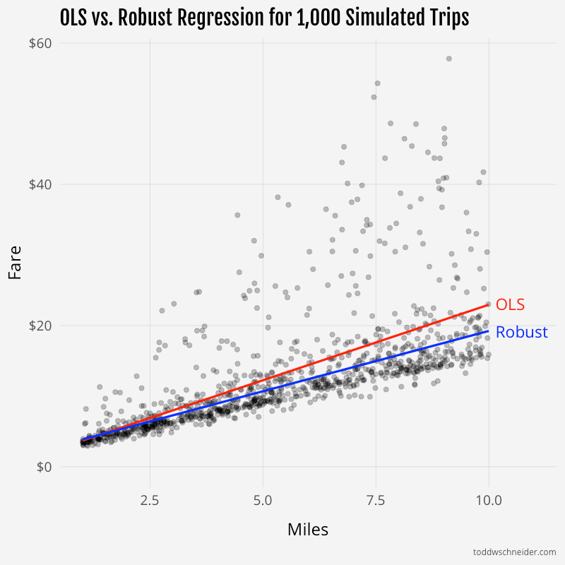
As something of a sanity check on the robust regression methodology, I simulated 1,000 trips with the following assumptions:
I then fit linear models of actual fare as a function of distance and time via ordinary least squares and robust methods. The robust model “recovered” the exact base fare parameters of $1.87, $0.82, and $0.27, while the OLS model fit parameters of $1.56, $1.00, and $0.35.
For the average simulated trip of 5.5 miles and 16.5 minutes, the OLS model predicts a fare of $12.79, 18% higher than the $10.84 fare predicted by the robust model. In some circumstances, the OLS model might be more useful. For example, if all you knew was that you were about to take a 5.5-mile, 16.5-minute trip in this simulated world, the OLS model represents the expected value of what you’re going to pay. But if you’re trying to decompose your payment into a base fare, surge multiplier, and discount, then the robust model is closer to the underlying truth. (Of course in this case we know the underlying truth because we created it; in real life we don’t have that luxury.)
You can see from the trendlines that the OLS model is “pulled” up by the outlier surge prices:
If you want to generate similar simulated data on your own, here’s some R code:
1 2 3 4 5 6 7 8 9 10 11 12 13 14 15 16 17 18 19 20 21 |
|
And again, all code used in this post is available on GitHub.
]]>I wrote some code to process the raw data, and built an interactive heatmap of 1.4 million collisions between July 2012 and January 2019. By default the color intensity represents the number of collisions in each area, but you can customize it to reflect injuries or fatalities.
Click here to view map in full screen or on a mobile device
Note that the raw data does not identify each collision with pinpoint accuracy, rather collisions are typically rounded to the nearest intersection, which makes some areas look artificially better or worse than they really are. For example, there are a number of collisions at both ends of the Verrazzano Bridge, but apparently none in between. In reality those collisions are likely spread more evenly across the bridge’s span, but the dataset rounds them to either the Brooklyn or Staten Island base.
The map shows the areas with the most injuries and fatalities, but I’m hesitant to use the phrase “most dangerous”, as the collisions data does not tell us how many motorists, cyclists, and pedestrians traveled through each area without injury. For example, more pedestrians are injured by motor vehicles in Times Square than in any other area, but Times Square probably has the most total pedestrians, so it’s possible that “pedestrian injuries per mile walked” is higher elsewhere. It might make for interesting further analysis to estimate total vehicle, bicycle, and pedestrian travel in each area, then attempt to calculate the areas with the highest probability of injury or fatality per unit of distance traveled.
Delancey Street on Manhattan’s Lower East Side accounts for the most cyclist injuries of any area. In November 2018, the city installed a new protected bike lane from the Williamsburg Bridge to Chrystie Street, and it will be interesting to see how effective it is in reducing future cyclist injuries. If the L train shutdown—in whatever form it ends up taking—causes more people to bike across the bridge, accidents and injuries might well increase, so as noted above, it will be important to adjust for total usage. The Manhattan base of the Queensboro Bridge also accounts for a significant number of cyclist injuries, and much like at the Williamsburg Bridge, there is an attempt underway to improve cycling conditions.
In Brooklyn, the areas with the most cyclist injuries include Grand Street between Union and Bushwick avenues in Williamsburg, and the section of Tillary Street between Adams and Jay streets downtown. In Queens, stretches of Roosevelt Avenue in Jackson Heights appear particularly dangerous. From Google Maps it appears that none of these three outer borough areas had fully protected bike lanes historically, though at least Grand Street’s bike lane was improved somewhat in the fall of 2018.
Google Street View illustrates some of the challenges cyclists face in these areas, including cars parked in bike lanes:
Tillary & Jay streets, Brooklyn
While I was working on this post, I happened to walk by Tillary & Jay streets one evening with some friends, one of whom captured this video of cyclists contending with a double-decker tour bus:
Video: Edwin Morris
Grand Street & Bushwick Avenue, Brooklyn
Roosevelt Avenue & 94th Street, Queens
I did not do any extensive investigation of the relationship between bike lanes and cyclist injuries, but it would make for interesting further analysis. The Department of Transportation publishes a city bike map along with a shapefile, and provides lists of active and past projects dedicated to bicycle safety, all of which could potentially be used to better understand the relationship between bike lane development and cyclist safety. At a minimum, it’s good to see that some of the areas with the most cyclist injuries have already been targeted for bike lane improvements.
As mentioned earlier, Times Square accounts for the most pedestrian injuries. Beyond Times Square and the Manhattan central business district more broadly, it looks like there might be a correlation between public transportation stations and pedestrian injuries. Outside of central Manhattan, several of the areas with the most pedestrian injuries are located near subway or rail stations, including:
I’d imagine that areas immediately surrounding subway stops have some of the highest rates of foot traffic, so it could be simply that more pedestrians equals more injuries. Or maybe subway stops tend to be located on busier, wider roads that are more dangerous to cross. It would be interesting to know if there are particular subway stations that have high or low pedestrian collision rates compared to their total usage, and if so, what features might distinguish them from other stations.
Motorist injuries are more geographically spread out than cyclist and pedestrian injuries, I would guess due to more vehicle travel at higher speeds in the outer boroughs compared to Manhattan. Highways look to account for many of the areas with the most motorist injuries: in the Bronx, sections of the Cross Bronx Expressway and Bronx River Parkway, along with the Van Wyck Expressway and Belt Parkway in Queens, and the western terminus of the Jackie Robinson Parkway in Brooklyn.
The city’s Vision Zero plan has the stated goal of eliminating all traffic deaths by the year 2024, and in general, traffic fatalities have been declining since 2012. One piece of confusion: the city recently announced that there were 200 traffic deaths city-wide in 2018, but the NYPD dataset reports 226 deaths in 2018. I’m not sure why those numbers are so different, but either way the trend still points toward decreasing fatalities.
The number of injuries per year has increased, though, and there are individual neighborhoods that have seen improving or worsening trends. To cherry-pick a few examples: Union Square, Chinatown, and East Harlem have seen some of the bigger reductions in injuries since 2012, while University Heights, Mott Haven, and East New York have seen injuries increase.
You can view trends city-wide, by borough, or by neighborhood (map) using the inputs below:
Note that the borough totals won’t necessarily add up to the city-wide total because about 5% of collisions are missing location data. The earlier data is more likely to be missing location data, which means that the graphs by borough are probably slightly pessimistic, and in reality the earlier years have a few more collisions and injuries relative to the recent years than otherwise stated. See this spreadsheet for a table of counts by borough and year, including collisions with unknown geography.
I’ve already noted a few potential topics for future work: population-adjusted collision rates and the impact of bike lanes/subway stations, but the dataset could be useful for many other analyses. Especially in the context of my previous post about taxi and Citi Bike travel times, I wonder about the relationship between increasing road congestion, slower average vehicle speeds, and fewer traffic-related fatalities.
Collisions are most common during daytime hours, when congestion is at its worst, but the likelihood of a collision resulting in an injury or fatality is highest during the late night/early morning hours. The dataset does not include detailed information about speed at the time of collision, but it seems likely that vehicles would be traveling faster at off-peak hours when there is less traffic. Darkness could also be an important factor, with differing effects on each of motorists, cyclists, and pedestrians.
The fatality rate is highest at 4 AM, which is last call for alcohol at NYC bars. The dataset includes contributing factors for each collision—albeit in a somewhat messy format—and sure enough the percentage of collisions involving alcohol also spikes at 4 AM:
Among collisions where alcohol is cited as a contributing factor, 30% result in an injury and 0.4% result in a fatality, compared to 19% and 0.1%, respectively, for collisions where alcohol is not cited. Many “correlation does not imply causation” caveats apply, including that alcohol involvement might be correlated with other factors that impact likelihood of injury, or there could be a bias in reporting alcohol as a factor given that the collision resulted in an injury or fatality.
I experimented a bit with regularized logistic regressions to model probability of injury and fatality as a function of several variables, including time of day, street type (avenue, street, highway, etc.), contributing factors, vehicle types, and more. The models consistently report a positive association between alcohol involvement and likelihood of injury and fatality, though in both cases the effect is not as strong as other factors like “unsafe speed” and “traffic control disregarded”. The model reports that collisions involving bicycles are the most likely to result in injuries, while collisions involving motorcycles are the most likely to result in fatalities. It will be interesting to see what happens if new vehicle types like electric scooters gain more widespread adoption.
Again the regression model cannot prove causation, but it’s still interesting to see which factors are most associated with injuries. The relevant code is available here on GitHub if you want to poke around more.
Population growth, gentrification, Citi Bike’s expansion, and various other traffic control mechanisms (speed limits, crosswalks, traffic lights, etc.) all come to mind as possible areas for further study, and kudos to the City of New York for making so much of the data publicly available.
The code used to collect and process the collisions data is available here on GitHub.
The interactive map is built with deck.gl and Mapbox.
The map embedded and linked in this post uses pre-aggregated data, which helps performance, but limits the number of filters available. If you want to go a bit deeper, there is a similar version of the map available here that aggregates on the fly, and therefore allows a few extra filters: time of day, number of vehicles involved, and injury status. Note though that this “on the fly” version is much slower to load, and likely will not work on mobile devices.
]]>The chart below shows how long you should expect to wait for each train line, assuming you arrive on the platform at a random time on a weekday between 7:00 AM and 8:00 PM.
The top four trains with the shortest waits—the L, 7, 1, and 6—are the only trains that run on dedicated tracks, which presumably helps avoid delays due to trains from other lines merging in and out on different schedules. The L train is also the only line that uses modern communications-based train control (CBTC), which allows trains to operate in a more automated fashion. The 7 train, the second most reliable according to my data, is currently running “partial” CBTC, and is slated for full CBTC in 2018.
Systemwide CBTC is the cornerstone of the recently announced ambitious plan to fix the subways. I’ll have a bit more to say on that in a moment…
(Note that expected wait time is different from time between trains. See the appendix for a more mathematical treatment on converting between time between trains and expected wait time. Note also that in some cases, different lines can serve as substitutes. For example, if you’re traveling from Union Square to Grand Central, the 4, 5, and 6 lines will all get you there, so your effective wait time would be shorter than if you had to rely on one specific line.)
The above graph is restricted to weekdays between 7:00 AM and 8:00 PM, but wait times vary from hour to hour. In general, wait times are shortest during morning and evening rush hours, though keep in mind that the data doesn’t know about cases where trains might be too crowded to board, forcing you to wait for the next train.
Choose your line below, and you can see how long you should expect to wait for a train by time of day, based on weekday performance from January to May 2018.
Most New Yorkers intuitively understand that when they get to a subway platform, they don’t want it to be too empty or too crowded. An empty platform means that you probably just missed the last train, so it’s unlikely another one will be arriving very soon. Even worse, an extremely crowded platform means that something is probably wrong, and maybe the train will never arrive. There’s a Goldilocks zone in the middle: a healthy amount of crowding that suggests it’s been a few minutes since the last train, but not so long that things must be screwed up.
I used the same data to compute conditional wait time distributions: given that it’s been N minutes since the last train, how much longer should you expect to wait? In most cases, the shortest conditional wait time occurs when it’s been 5 to 8 minutes since the last train.
Choose your line to view conditional wait times.
In general when you arrive on the platform, you can’t directly observe when the last train departed, but you can make a guess based on the number of people who are waiting. First you would have to estimate—or maybe even measure from the MTA’s public turnstile data—the number of people who arrive on the platform each minute. Then, if you know the shortest conditional wait occurs when it’s been 6 minutes since the last train, and you estimated that, say, 20 people arrive on the platform each minute, you should hope to see 120 people on the platform when you arrive. Of course these parameters vary by platform and time of day, so make sure to take that into account when making your own estimates!
The recently released Fast Forward plan from Andy Byford, president of the NYC Transit Authority, proposes that it will take 10 years to implement CBTC across most of the system. The NYT further reports an estimated price tag of $19 billion.
If every line were as efficient as the CBTC-equipped L, I estimate that the average wait time would be around 3 minutes shorter. At 5.7 million riders per weekday, that’s potentially 285,000 hours of time saved per weekday. Reasonable people might disagree about the economic value of deadweight subway waiting time, but $20 per hour doesn’t strike me as crazy, and would imply a savings of $5.7 million per weekday. Weekends have about half as many riders as weekdays, and time is probably worth less, so let’s value a weekend day’s savings at 25% of a weekday’s.
Overall that would imply a total savings of over $1.6 billion per year, and that’s before accounting for the fact that CBTC-equipped trains also probably travel faster from station to station, so time savings would come from more than reduced platform wait times. And if people had more confidence in the system, they wouldn’t have to budget so much extra travel time as a safety buffer. Other potential benefits could come from lower operating and repair costs, and less above-ground traffic congestion if people switched from cars to the presumably more efficient subway.
To be fair, there are all kinds of things that could push in the other direction too: maybe it’s unrealistic that other lines would be as efficient as the L, since the L has the benefit of being on its own dedicated track that it doesn’t share with any other crisscrossing lines, or maybe the better subway would be a victim of its own success, causing overcrowding and other capacity problems. And perhaps the most obvious criticism: that the plan will end up taking longer than 10 years and costing more than $19 billion.
I don’t think this quick back-of-the-envelope calculation should be taken too seriously when there are so many variables to consider, but I do think it’s not hard to get to a few billion dollars a year in economic value, assuming some reasonable parameters. Reasonable people might again argue about discount rates and amortization schedules, but a total cost in the neighborhood of $19 billion over 10 years strikes me as eminently worth it.
The NYT recently published a great interactive story that demonstrated via simulation how a single train delay can cause cascading problems behind it. The week after that story was published, I was (un)fortunate enough to participate in a real-life demonstration of the phenomenon. On May 16, 2018, I found myself on a downtown F train from Midtown. Around 10:00 AM at 34th Street, the conductor made an announcement that there was a stalled train in front of us at W 4th Street, and that we’d be delayed. The delay lasted about 30 minutes, and then the train carried on as normal.
Here’s a graphical representation of downtown F trains that morning, with major delays highlighted in red. My train was the second train in the major delay on the right-center of the graph.
Although I wasn’t on the train that had mechanical problems at W 4th Street, my train and the two trains behind it were forced to wait for the problem train. Further back, the train dispatcher switched a few F trains to the express tracks from 47-50 Sts–Rockefeller Center to W 4th Street, which is why you see a few steeper line segments in the graph that appear to cut through the delay. The empty diagonal gash in the graph below the delay shows that riders felt the effects all the way down the line. If you were waiting for an F train at 2nd Avenue just after 10:00 AM, you would have had to wait a full 30 minutes, compared to only a few minutes if you had arrived on the platform at 9:55 AM.
I’m a bit surprised that the MTA didn’t deliberately slow down some of the trains in front of the delay. It’s well-known that even spacing is a key to minimizing system-wide wait time, the MTA once even made a video about it, but in this case it appears they didn’t practice what they preach. Slowing down a train in front of a delay will make some riders worse off, namely the ones at future stops who would have made the train had it not been slowed down. But it will also make some riders much better off: the ones who would have missed the train had it not been slowed down, and then had to suffer an abnormally long wait for the delayed train itself.
You can use the graph to convince yourself that slowing down the train ahead of the delay would have been a good thing. Downtown F trains stopped at 2nd Avenue at 9:58 and 10:00 AM. If the 10:00 AM train had been intentionally delayed 10 minutes to 10:10 AM, all of the people who arrived on the platform between 10:00 and 10:10 would have been saved from waiting until 10:30, an average 20 minute savings per person. On the other hand, the folks who arrived between 9:58 and 10:00 would have been penalized an average of 10 minutes per person. But there were likely five times as many people in the 10:00–10:10 range than there were in the 9:58–10:00 range, so the weighted average tells us we just saved an average of 15 minutes per person.
Compare the W 4th Street delay to the delay earlier that morning at 7:40 AM at 57th Street, highlighted on the left side of the graph. That delay, although shorter, also caused a lasting gap between trains. However, the gap was later mitigated when the train in front of the delayed train slowed down a bit between York and Jay streets. I suspect that slowdown was unintentional, but it was probably beneficial, and had it happened further up the line, say between 42nd and 34th streets, it would have produced more even spacing throughout the line, and likely lowered total rider wait time.
In fairness to the MTA, in real life it’s not as simple as “always slow down the train in front of the delay” because there are other considerations—dispatchers don’t know how long the delay will last, not every platform is equally popular, and there other options like rerouting trains to other tracks—but a healthier system could have dealt with this delay better.
The subway’s deteriorating performance has been covered at great length by many outlets. I’d recommend the NYT’s coverage in particular, but it seems like there are so many people writing about the subway recently that there’s no shortage of stories to choose from.
In addition to the dataset I collected starting in January 2018, the MTA makes some real-time snapshots available going back to September 2014. These snapshots are only available for the 1, 2, 3, 4, 5, 6, and L trains, and they’re in 5-minute increments as opposed to the 1-minute increments of my tracker. Additionally, there is a gap in historical coverage from November 2015 until January 2017.
The historical data shows that expected wait times have remained fairly unchanged since 2014, but travel times from station to station have gotten a bit slower, at least on the 2, 3, 4, and 5 trains, where a weekday daytime trip in 2018 takes 3-5% longer on average than the same trip in 2014. The 1 and 6 trains have not experienced similar slowdowns, and the L is somewhere in the middle.
On a 15-minute trip, 3-5% is an average of 30-45 seconds slower, which doesn’t sound particularly catastrophic, but there are plenty of other issues not reflected in these numbers that might make the subway “better” or “worse” over time. I’ve tried to exclude scheduled maintenance windows from the expected wait time calculations, but in reality scheduled maintenance and station closures can be a huge nuisance. The MTA data also doesn’t tell us anything about when trains are so crowded that they can’t pick up new passengers, when air conditioning systems are broken, and other general quality-of-ride characteristics.
It’s also possible that the 1-6 and L lines—the ones with historical data—happen to have deteriorated less than the other lettered lines, and if we had full historical data for the other lines, we’d see more dramatic effects over time. There’s no question that the popular narrative is that the subway has gotten worse in recent years, though part of me can’t help but wonder if the feedback loop provided by nonstop media coverage might be a contributing factor…
I used the igraph package in R to construct a weighted directed graph of the subway system, where the nodes are the 472 subway stations, the edges are the various subway lines and transfers that connect them, and the weights are the expected travel times along each edge. For train edges, the weight is calculated as the median wait time on the platform plus the median travel time from station to station, and for transfer edges, the weight is taken from estimates provided by the MTA—typically 3 minutes if you have to change platforms, 0 if you don’t.
With the graph in hand, we can answer a host of fun (and maybe informative) questions, as igraph does the heavy lifting to calculate shortest possible paths from station to station across the system.
I used the directed graph to find the “center” of the subway system, defined as the station that has the closest farthest-away station. That honor goes to the Chambers Street–World Trade Center/Park Place station, from where you can expect to reach any other subway station in 75 minutes or less. Here’s a map highlighting the Chambers Street station, plus the routes you could take to the farthest reaches of Manhattan, Brooklyn, Queens, and the Bronx.
The directed graph might even be a good real estate planning tool. You might not care about the outer extremities of the city, but if you provide a list of neighborhoods you do frequent, the graph can tell you the most central station where you can minimize your worst-case travel times.
For example, if your personal version of NYC stretches from the Upper West Side to the north, Park Slope to the south, and Bushwick to the east, then the graph suggests W 4th Street in Greenwich Village as your subway center: you can get to all of your neighborhoods in a maximum of 26 minutes.
The graph can be used to calculate all sorts of other fun routes. I’ve seen attempts to find the longest possible subway trip that doesn’t involve any backtracking, which is all well and good, but what about finding the longest trip from A to B with the constraint that it’s also the fastest subway-only trip from A to B? Based on my calculations, the longest possible such trip stretches from Wakefield–241st Street in the Bronx to Far Rockaway–Beach 116th Street in Queens via the 2, 5, A, and Rockaway Park Shuttle. It would take a median time of 2:28—about as long as it takes the Acela to travel from Penn Station to Baltimore.
The fastest way to hit all 4 subway boroughs is from 138th St–Grand Concourse in the South Bronx to Greenpoint Avenue in North Brooklyn: 41 minutes via the 6, 4, E, and G trains. And the “centers” of each borough:
The directed graph is a bit silly: in many cases it wouldn’t make sense to rely only on the subway when other transportation options would be more sensible. I’ve written previously about taxi vs. Citi Bike travel times, and a logical extension would be to expand the edges of the directed graph to take into account more transportation options.
Of course, a more practical idea might be to use Google Maps travel time estimates, which already do some of the work combining subways, bikes, ferries, buses, cars, and walking. Still, there’s something nice about estimating travel times based on historical trips that actually happened, as opposed to using posted schedules.
There’s probably something interesting to learn by combining the MTA’s public turnstile data with the train location data. For example, the turnstiles might provide insights into when dispatchers should be more aggressive about maintaining even train spacing following delays. As the tracker collects more data, it might be interesting to see how weather affects subway performance, perhaps segmenting by routes that are above or below ground.
All eyes will be on the subway system in the months and years to come, as people wait to see how the current “fix the subway” drama unfolds. Hopefully the MTA’s real-time data can serve as a resource to measure progress along the way.
Although there’s no official record of when trains actually stopped at each station, the MTA provides a public API of the real-time data that powers the countdown clocks, which can be used to estimate train performance.
Starting in January 2018, I’ve been collecting the countdown clock information every minute for every line in the NYC subway system, then calculating my best guesses as to when each train stopped at each station. Between January and May 2018, I observed some 900,000 trains that collectively made 24 million stops. The MTA’s data is very messy, and occasionally makes no sense at all, so I spent a considerable amount of time trying to clean up the data as best possible. For more technical details, including all of the code used in this post to collect and analyze the data, head over to GitHub.
The countdown clock system uses bluetooth receivers installed on trains and in stations: when a train passes through a station, it notifies the system of its most recent stop. The MTA has acknowledged the system’s less than perfect accuracy, but it’s much better than the status quo from only a few years ago when we really had no idea where the trains were.
Putting aside messy data issues, the MTA’s real-time feeds tell us the amount of time between trains. But riders probably care more about how long they should expect to wait when they arrive at the platform, and those two quantities can be different.
As a hypothetical example, imagine a system where trains arrive exactly every 10 minutes on the 0s: 12:00, 12:10, etc. In that world, riders who arrive on the platform at 12:01 will wait 9 minutes for the next train, riders who arrive at 12:02 will wait 8 minutes, and so on down to riders who arrive at 12:09 who will wait 1 minute. If we assume a continuous uniform distribution of arrival times for people on the platform, the average person’s wait time will be one half of the time between trains, 5 minutes in this example.
Now imagine trains arrive alternating 5 and 15 minutes apart, e.g. 12:00, 12:05, 12:20, 12:25, etc., while people still arrive following a uniform distribution. The people who happen to arrive during one of the 5-minute gaps will average a 2.5 minute wait, while the people who arrive during one of the 15-minute gaps will average a 7.5 minute wait. The catch is that only 25% of all people will arrive during a 5-minute window while the other 75% will arrive during a 15-minute window, which means the global average wait time is now (2.5 * 0.25) + (7.5 * 0.75) = 6.25 minutes. That’s 1.25 minutes worse than the first scenario where trains were evenly spaced, even though in both scenarios the average time between trains is 10 minutes.
If you work out the math for the general case, you should find that average wait time is proportional to the sum of the squares of each individual gap between trains.
This means that given an average gap time, expected wait time will be minimized when the gaps are all identical. In practice, it very well could be worth increasing average gap time if it means you can minimize gap time variance. Looking back to our toy example, not only is the average of 52 and 152 greater than 102, it’s greater than 112, which means that trains spaced evenly every 11 minutes will produce less average wait time than trains alternating every 5 and 15 minutes, even though the latter scenario would have a shorter average gap between trains. For another take on this, I’d recommend Erik Bernhardsson’s NYC subway math post from 2016.
Often we want more than the expected wait time, we want the distribution of wait times, so that we can calculate percentile outcomes. Normally this is where I’d say something like “just write a Monte Carlo simulation”, but I think in this particular case it’s actually easier and more useful to do the empirical calculation.
Let’s say you have a list of the times at which trains stopped at a particular station, and you’d like to calculate the empirical distribution of rider wait times, assuming riders arrive at the platform following a uniform distribution. I’d reframe that problem as drawing balls out of a box, following the process below:
Once you’ve done that, you’re pretty much done, as your box is now full of balls with numbers on them, and the probability of a rider having to wait some specific number of seconds t is equal to the number of balls labeled t divided by the total number of balls in the box. Note that you might want to filter trains by day of week or time of day, both because train schedules vary, and people don’t actually arrive on platforms uniformly, but if you restrict to within narrow enough time intervals, it’s probably close enough.
In terms of the actual NYC subway lines during weekdays between 7:00 AM and 8:00 PM, the 7 train has the shortest median time between trains, but the L does a better job at minimizing the occasional long gaps between trains, which is why we saw earlier that the L has shorter average wait times than the 7.
The A train has a notably flat and wide distribution, which explains why the first graph in this post showed that the A had the worst 75th and 90th percentile outcomes, even though its median performance is middle-of-the-pack.
]]>Shot data has some significant limitations, and we should be very wary of drawing unjustified conclusions from it, but it can also help illuminate trends that might not be otherwise obvious to the human eye.
The NBA’s aggregate field goal percentage is slightly better than the NCAA’s, 46% to 44%. I would have guessed that NBA professionals would be better shooters than NCAA players at all distances, but it turns out that for shots under 6 feet, NCAA attempts are more likely to go in. The shot data can’t tell us why—my guess is that the NCAA has more mismatches where an offensive player is much bigger than his defender, leading to easier interior shots, but we don’t really know.
An important disclaimer: neither dataset is particularly clear about where its data comes from. The NBA data is presumably generated by the SportVU camera systems installed at NBA arenas, but I don’t know how Sportradar produces the NCAA data. It could come from cameras, manual review of game tape, or something else. If the systems that gather the data are different enough, it might make comparisons less meaningful.
For example, it seems a bit odd that the NBA data reports a much higher frequency of shots less than 1 foot from the basket. It makes me think the measurement systems might be different, and maybe what’s recorded as a “1 foot” shot in the NBA is recorded as a “3 foot” shot in the NCAA. If we restrict to all shots under 6 feet in each dataset, the NCAA still has a slightly higher FG% than the NBA (59% vs. 58%), but depending on how the recording systems work, the accuracy gap at short distances might be significantly smaller than the graph would have you believe.
The college 3-point line is 3 feet closer to the basket than the NBA line in most places, though the gap narrows to 1.25 feet in the corners. But of course there’s nothing to stop a college player from shooting from NBA 3-point range, and NBA scouts might be particularly interested in how college players shoot from NBA-range as a predictor of future pro performance.
I used the Sportradar NCAA data to isolate shots that were not only 3-pointers, but would have been 3-pointers even in the NBA, then ranked college players by their NBA-range 3-point accuracy. Here’s a list of NCAA players who attempted at least 100 NBA-range 3-pointers since 2013:
Unfortunately for any aspiring scouts, it looks like this might not be a good predictor of future NBA performance. Based on the 23 players in the dataset who attempted at least 100 NBA-range 3-pointers in college and another 100 3-pointers in the NBA, there’s no strong correlation between college and pro results. Most of the players had lower accuracy in the NBA than in college, though Terry Rozier of Louisville and the Boston Celtics managed to improve his NBA-range 3-point shooting by +9%.
There are many competing factors that might influence field goal accuracy when a player transitions from college to the pros. Players presumably get better with age in their early 20s as they mature physically, NBA players probably practice more, and have access to better training facilities and coaching, all of which suggest they might shoot better in their first professional season than they did in college. On the other hand, NBA rookies have to play against other NBA players, who are on average much better defenders than their previous college opponents.
We’ve seen anecdotally with 3-point attempts that an individual player usually shoots worse in the NBA than he did in college, but I wanted to do something at least a bit more scientific to quantify the effect. Using a dataset of 129,000 shots from 262 players who appear in both datasets, I ran a logistic regression to estimate the change in field goal accuracy associated with the transition from college to the NBA. It’s a crude model, considering shot distance, whether the player is in his final year of college or his first year in the NBA, and a player-level adjustment for each player. The model ignores any differences between positions, so if guards and centers are affected differently, the model would probably miss it.
The simple model predicts that, on average, as a player goes from his last year in college to his first year in the NBA, his field goal percentage will decline by around 4% on shots over 6 feet, and as much as 15% on shorter shots. It doesn’t say anything about why, though again I’d suspect the primary explanation is that NBA players are much better defenders.
At first glance, this result that players shoot worse when they go from college to the NBA might seem in conflict with the first chart in this post, which showed that NBA players had higher field goal percentages on longer shots than college players. The most likely explanation is that rookies are below-average shooters among all NBA players, and as rookies turn into veterans, their shooting performance improves. Note that the merged NBA/NCAA dataset has a data truncation issue: because the NCAA data only spans 2013–18, any player who was in both leagues during that period has at most 4 years of NBA experience. Over time, assuming both datasets remain publicly available, it will be interesting to see if there is an NBA experience level where a player’s shooting performance is expected to exceed his college stats.
Even the most casual basketball fan probably knows by now that 3-point attempts have exploded in popularity, while mid-range 2-point attempts are in decline. It’s gotten to the point where there are some signs of blowback, but overall the trend continues.
The NBA Stats API provides some aggregate data on shooting performance based on both the distance of the shot, and the distance of the closest defender at the time of the shot, which shows that yes, usually a 3-point attempt has a higher expected value than a long-range 2. But if the 3-pointer is tightly guarded and the long-range 2 is wide-open, then the 2-pointer can be better. For example, a wide-open 2-point shot from 20 feet on average results in 0.84 points, while a tightly-guarded 3-point attempt from 25 feet only averages 0.71 points.
The same table, in graph form:
Again, basketball is complicated and these isolated data points are not a final authority on what constitutes a good or bad shot. In the 2017-18 season, the Houston Rockets and Indiana Pacers have both been successful even though they are at opposite ends of the shooting spectrum, with the Rockets shooting the most 3s, and the Pacers shooting the most long-distance 2s. To be fair, the 3-point-happy Rockets currently have the best record in the league, but the Pacers’ success, despite taking the most supposedly “bad” mid-range 2s of any team in the league, suggests that there’s more than one way to win a basketball game.
Another important note: for unknown reasons, the aggregate stats by distance and closest defender do not match the aggregates computed from the individual shot-level data. The shot-level data includes more attempts, which makes me think that the aggregates by closest defender are somehow incomplete, but I wasn’t able to find more information about why. The difference is particularly pronounced in shots of around 4 feet, with the shot-level data reporting a significantly lower FG% than the aggregate data.
The code used to compile and analyze all of the NBA and NCAA shots is available here on GitHub. The NBA Stats API has many more (mostly undocumented) endpoints, and the code could probably be expanded to capture more information that could feed into more detailed analysis.
Every so often I see a story about whether or not the hot-hand exists, and though I kind of doubt that debate will ever be settled conclusively, maybe the shot-collecting code can be of use to future researchers.
The Los Angeles Times made a nice graphic of all 30,000+ shots Kobe Bryant ever attempted in the NBA, and you could use the data in NBA Shots DB to do something similar for any NBA player since 1996. Here’s an image of every shot LeBron James has attempted during his NBA career:
Or you could do a team-level analysis, for example comparing the aforementioned Houston Rockets (lots of 3-pointers) to the Indiana Pacers (lots of mid-range 2-pointers):
These images use an adapted version of my BallR shot chart app, but a better solution would be to expose an API from the NBA Shots DB app, then have BallR connect to that API instead of hitting the NBA Stats API directly.
]]>The methodology and findings will be explained more below, and all code used in this post is available open-source on GitHub.
Pick a starting neighborhood and a time. The map shows whether you’d expect get to each neighborhood faster with a taxi (yellow) or a Citi Bike (dark blue).
Taxi vs. Citi Bike travel times to other neighborhoods
Hover over a neighborhood (tap on mobile) to view travel time stats
I estimate that 40% of weekday taxi trips within the Citi Bike service area would expect to be faster if switched to a Citi Bike, based on data from July 2016 to June 2017. During peak midday hours, more than 50% of taxi trips would expect to be faster as Citi Bike rides.
There are some significant caveats to this estimate. In particular, if many taxi riders simultaneously switched to Citi Bikes, the bike share system would probably hit severe capacity constraints, making it difficult to find available bikes and docks. Increased bike usage might eventually lead to fewer vehicles on the road, which could ease vehicle congestion, and potentially increase bike lane congestion. It’s important to acknowledge that when I say “40% of taxi trips would be faster if they switched to Citi Bikes”, we’re roughly considering the decision of a single able-bodied person, under the assumption that everyone else’s behavior will remain unchanged.
Crosstown Manhattan trips are generally regarded as more difficult than their north-south counterparts. There are fewer subways that run crosstown, and if you take a car, the narrower east-west streets often feel more congested than the broad north-south avenues with their synchronized traffic lights. Crosstown buses are so notoriously slow that they’ve been known to lose races against tricycles.
I divided Manhattan into the crosstown zones pictured above, then calculated the taxi vs. Citi Bike win rate for trips that started and ended within each zone. Taxis fare especially badly in the Manhattan central business district. If you take a midday taxi that both starts and ends between 42nd and 59th streets, there’s over a 70% chance that the trip would have been faster as a Citi Bike ride.
Keep in mind that’s for all trips between 42nd and 59th streets. For some of the longest crosstown routes, for example, from the United Nations on the far east side to Hell’s Kitchen on the west, Citi Bikes beat taxis 90% of the time during the day. It’s worth noting that taxis made 8 times as many trips as Citi Bikes between 42nd and 59th streets from July 2016 to June 2017—almost certainly there would be less total time spent in transit if some of those taxi riders took bikes instead.
Hourly graphs for all of the crosstown zones are available here, and here’s a summary table for weekday trips between 8:00 AM and 7:00 PM:
Manhattan crosstown zone | % taxis lose to Citi Bikes |
---|---|
96th–110th | 41% |
77th–96th | 36% |
59th–77th | 54% |
42nd–59th | 69% |
14th–42nd | 64% |
Houston–14th | 54% |
Canal–Houston | 60% |
Below Canal | 55% |
A reminder that this analysis restricts to trips that start and end within the same zone, so for example a trip from 23rd St to 57th St would be excluded because it starts and ends in different zones.
Taxis fare better for trips that stay on the east or west sides of Manhattan: 35% of daytime taxi trips that start and end west of 8th Avenue would expect to be faster as Citi Bike trips, along with 38% of taxi trips that start and end east of 3rd Avenue. Taxis also generally beat Citi Bikes on longer trips:
When the Citi Bike program began in July 2013, less than half of weekday daytime taxi trips would have been faster if switched to Citi Bikes. I ran a month-by-month analysis to see how the taxi vs. Citi Bike calculus has changed over time, and discovered that taxis are getting increasingly slower compared to Citi Bikes:
Note that this month-by-month analysis restricts to the original Citi Bike service area, before the program expanded in August 2015. The initial expansion was largely into Upper Manhattan and the outer boroughs, where taxis generally fare better than bikes, and so to keep things consistent, I restricted the above graph to areas that have had Citi Bikes since 2013.
Taxis are losing more to Citi Bikes over time because taxi travel times have gotten slower, while Citi Bike travel times have remained roughly unchanged. I ran a pair of linear regressions to model travel times as a function of:
The regression code and output are available on GitHub: taxi, Citi Bike
As usual, I make no claim that this is a perfect model, but it does account for the basics, and if we look at the coefficients by year, it shows that, holding the other variables constant, a taxi trip in 2017 took 17% longer than the same trip in 2009. For example, a weekday morning trip from Midtown East to Union Square that took 10 minutes in 2009 would average 11:45 in 2017.
The same regression applied to Citi Bikes shows no such slowdown over time, in fact Citi Bikes got slightly faster. The regressions also show that:
It’s one thing to say that 50% of midday taxi trips would be faster as Citi Bike rides, but how much does that vary from day to day? You could imagine there are some days with severe road closures, where more nimble bikes have an advantage getting around traffic, or other days in the dead of summer, when taxis might take advantage of the less crowded roads.
I ran a more granular analysis to measure win/loss rates for individual dates. Here’s a histogram of the taxi loss rate—the % of taxi trips we’d expect to be faster if switched to Citi Bikes—for weekday afternoon trips from July 2016 to June 2017:
Many days see a taxi loss rate of just over 50%, but there are tails on both ends, indicating that some days tilt in favor of either taxis or Citi Bikes. I was curious if we could learn anything from the outliers on each end, so I looked at individual dates to see if there were any obvious patterns.
The dates when taxis were the fastest compared to Citi Bikes look like dates that probably had less traffic than usual. The afternoon with the highest taxi win rate was Monday, October 3, 2016, which was the Jewish holiday of Rosh Hashanah, when many New Yorkers would have been home from work or school. The next 3 best days for taxis were all Mondays in August, when I’d imagine a lot of people were gone from the city on vacation.
The top 4 dates where Citi Bikes did best against taxis were all rainy days in the fall of 2016. I don’t know why rainy days make bikes faster relative to taxis, maybe rain causes traffic on the roads that disproportionately affects cars, but it’s also possible that there’s a selection bias. I’ve written previously about how the weather predicts Citi Bike ridership, and not surprisingly there are fewer riders when it rains. Maybe the folks inclined to ride bikes when it’s raining are more confident cyclists, who also pedal faster when the weather is nice. It’s also possible that rainy-day cyclists are particularly motivated to pedal faster so they can get out of the rain. I don’t know if these are really the causes, but they at least sound believable, and would explain the observed phenomenon.
June 8, 2016 was a particularly good day for Citi Bikes compared to taxis. President Obama came to town that afternoon, and brought the requisite street closures with him. I poked around a bit looking for the routes that appeared to be the most impacted by the President’s visit, and came to afternoon trips from Union Square to Murray Hill. On a typical weekday afternoon, taxis beat Citi Bikes 57% of the time from Union Square to Murray Hill, but on June 8, Citi Bikes won 90% of the time. An even more dramatic way to see the Obama effect is to look at daily median travel times:
A typical afternoon taxi takes 8 minutes, but on June 8, the median was over 21 minutes. The Citi Bike median travel time is almost always 9 minutes, including during President Obama’s visit.
The same graph shows a similar phenomenon on September 19, 2016, when the annual United Nations General Assembly shut down large swathes of Manhattan’s east side, including Murray Hill. Although the impact was not as severe as during President Obama’s visit, the taxi median time doubled on September 19, while the Citi Bike median time again remained unchanged.
The morning of June 15, 2016 offers another example, this time on the west side, when an overturned tractor trailer shut down the Lincoln Tunnel for nearly seven hours. Taxi trips from the Upper West Side to West Chelsea, which normally take 15 minutes, took over 35 minutes. Citi Bikes typically take 18 minutes along the same route, and June 15 was no exception. Taxis would normally expect to beat Citi Bikes 67% of the time on a weekday morning, but on June 15, Citi Bikes won over 92% of the time.
These are of course three hand-picked outliers, and it wouldn’t be entirely fair to extrapolate from them to say that Citi Bikes are always more resilient than taxis during extreme circumstances. The broader data shows, though, that taxis are more than twice as likely as Citi Bikes to have days when a route’s median time is at least 5 minutes slower than average, and more than 3.5 times as likely to be at least 10 minutes slower, so it really does seem that Citi Bikes are better at minimizing worst-case outcomes.
The biggest slowdowns in taxi travel times happened in 2014 and 2015. The data and regression model have nothing to say about why taxis slowed down so much over that period, though it might be interesting to dig deeper into the data to see if there are specific regions where taxis have fared better or worse since 2009.
Uber usage took off in New York starting in 2014, reaching over 10,000 vehicles dispatched per week by the beginning of 2015. There are certainly people who blame Uber—and other ride-hailing apps like Lyft and Juno—for increasing traffic, but the city’s own 2016 traffic report did not blame Uber for increased congestion.
It’s undoubtedly very hard to do an accurate study measuring ride-hailing’s impact on traffic, and I’m especially wary of people on both sides who have strong interests in blaming or exonerating the ride-hailing companies. Nevertheless, if I had to guess the biggest reasons taxis got particularly slower in 2014 and 2015, I would start with the explosive growth of ride-hailing apps, since the timing looks to align, and the publicly available data shows that they account for tens of thousands of vehicles on the roads.
On the other hand, if ride-hailing were the biggest cause of increased congestion in 2014 and 2015, it doesn’t exactly make sense that taxi travel times have stabilized a bit in 2016 and 2017, because ride-hailing has continued to grow, and while taxi usage continues to shrink, the respective rates of growth and shrinkage are not very different in 2016–17 than they were in 2014–15. One explanation could be that starting in 2016 there was a reduction in other types of vehicles—traditional black cars, private vehicles, etc.—to offset ride-hailing growth, but I have not seen any data to support (or refute) that idea.
There are also those who blame bike lanes for worsening vehicle traffic. Again, different people have strong interests arguing both sides, but it seems like there are more data points arguing that bike lanes do not cause traffic (e.g. here, here, and here) than vice versa. I wasn’t able to find anything about the timing of NYC bike lane construction to see how closely it aligns with the 2014–15 taxi slowdown.
Lots of other factors could have contributed to worsening traffic: commuter-adjusted population growth, subway usage, decaying infrastructure, construction, and presidential residences are just a few that feel like they could be relevant. I don’t know the best way to account for all of them, but it does seem like if you want to get somewhere in New York quickly, it’s increasingly less likely that a car is your best option.
I think it’s not a terrible assumption that taxis are representative of typical car traffic in New York. If anything, maybe taxis are faster than average cars since taxi drivers are likely more experienced—and often aggressive—than average drivers. On the other hand, taxi drivers seem anecdotally less likely to use a traffic-enabled GPS, which maybe hurts their travel times.
Citi Bikes are probably slower than privately-owned bikes. Citi Bikes are designed to be heavy and stable, which maybe makes them safer, but lowers their speeds. Plus, I’d guess that biking enthusiasts, who might be faster riders, are more likely to ride their own higher-performance bikes. Lastly, Citi Bike riders might have to spend extra time at the end of a trip looking for an available dock, whereas privately-owned bikes have more parking options.
Weighing up these factors, I would guess that if we somehow got the relevant data to analyze the broader question of all cars vs. all bikes, the results would tip a bit in favor of bikes compared to the results of the narrower taxi vs. Citi Bike analysis. It’s also worth noting that both taxis and Citi Bikes have additional time costs that aren’t accounted for in trip durations: you have to hail a taxi, and there might not be a Citi Bike station in the near vicinity of your origin or destination.
One thing to keep in mind is that even though the taxi and Citi Bike datasets are the most conveniently available for analysis, New Yorkers don’t limit their choices to cars and bikes. The subway, despite its poor reputation of late, carries millions of people every day, more than taxis, ride-hailing apps, and Citi Bikes combined, so it’s not like “car vs. bike” is always the most relevant question. There are also legitimate reasons to choose a car over a bike—or vice versa—that don’t depend strictly on expected travel time.
Bike usage in New York has increased dramatically over the past decade, probably in large part because people figured out on their own that biking is often the fastest option. Even with this growth, though, the data shows that a lot of people could still save precious time—and minimize their worse-case outcomes—if they switched from cars to bikes. To the extent the city can incentivize that, it strikes me as a good thing.
For any readers who might be affected by the L train’s planned 2019 closure, if you only remember one thing from this post: Citi Bikes crush taxis when traveling from Williamsburg to just about anywhere in Manhattan during morning rush hour!
The code for the taxi vs. Citi Bike analysis is available here as part of the nyc-taxi-data repo. Note that parts of the analysis also depend on loading the data from the nyc-citibike-data repo.
Taxi trip data is available since January 2009, Citi Bike data since July 2013. I filtered each dataset to make the analysis closer to an apples-to-apples comparison—see the GitHub repo for a more complete description of the filtering—but in short:
Starting in July 2016, perhaps owing to privacy concerns, the TLC stopped providing latitude and longitude coordinates for every taxi trip. Instead, the TLC now divides the city into 263 taxi zones (map), and provides the pickup and drop off zones for every trip. The analysis then makes the assumption that taxis and Citi Bikes have the same distribution of trips within a single zone, see GitHub for more.
80% of taxi trips start and end within zones that have Citi Bike stations, and the filtered dataset since July 2013 contains a total of 330 million taxi trips and 27 million Citi Bike trips. From July 1, 2016 to June 30, 2017—the most recent 12 month period of available data—the filtered dataset includes 68 million taxi trips and 9 million Citi Bike trips.
I wrote a Monte Carlo simulation in R to calculate the probability that a Citi Bike would be faster than a taxi for a given route. Every trip is assigned to a bucket, where the buckets are picked so that trips within a single bucket are fairly comparable. The bucket definitions are flexible, and I ran many simulations with different bucket definitions, but one sensible choice might be to group trips by:
For example, weekday trips from the West Village to Times Square between 9:00 AM and 10:00 AM would constitute one bucket. The simulation iterates over every bucket that contains at least 5 taxi and 5 Citi Bike trips, and for each bucket, it draws 10,000 random samples, with replacement, for each of taxi and Citi Bike trips. The bucket’s estimated probability that a taxi is faster than a Citi Bike, call it the “taxi win rate”, is the fraction of samples where the taxi duration is shorter than the Citi Bike duration. You can think of this as 10,000 individual head-to-head races, with each race pitting a single taxi trip against a single Citi Bike trip.
Different bucketing and filtering schemes allow for different types of analysis. I ran simulations that bucketed by month to see how win rates have evolved over time, simulations that used only days where it rained, and others. There are undoubtedly more schemes to be considered, and the Monte Carlo methodology should be well equipped to handle them.
]]>The Chicago dataset does not include data from ridesharing companies like Uber and Lyft, but the data makes clear that taxi usage in Chicago has declined dramatically since 2014. As of November 2016, Chicago taxi usage was declining at a 35% annual rate, and had fallen a cumulative 55% since peaking in June 2014.
Again, the public dataset does not include any data from ridesharing services like Uber and Lyft, but the Chicago taxi industry claims that ridesharing services caused cabs to lose 30–40% of their business in the summer of 2015.
New York taxis have also been losing market share to ridesharing companies—NYC releases data that confirms this—but in fact Chicago taxis are losing market share even faster than their NYC counterparts. While NYC taxi usage has been declining at around 10% per year, Chicago’s declines have reached 35% year-over-year.
New York taxis make about 8 times more trips per month than Chicago taxis do, but a rescaled monthly trips index shows that Chicago has a larger cumulative decline on a percentage basis.
Chicago’s taxi pickup declines are not evenly distributed among the city’s 77 community areas. For example, the Loop, Chicago’s central business district, shows a 23% annual decline, while Logan Square on the northwest side shows a 50% annual decline. In general, the areas located closest to the central business district show smaller declines in taxi activity.
I defined 5 particular community areas—the Loop, Near North Side, Near West Side, Near South Side, and O’Hare Airport—as the “core”, then compared pickups inside and outside of the core. As of November 2016, pickups inside the core show a 27% annual decline compared to a 42% annual decline outside of the core. On a cumulative basis, core pickups have declined 39% since June 2014, while non-core pickups have declined a whopping 65%. The smaller taxi decline near the central business district is consistent with NYC’s taxi and Uber data, where taxi share has fallen less in Manhattan than in the outer boroughs.
Data by community area is available here in spreadsheet form.
A map of the official community area definitions is available here, and you can select community areas in the menu below to view taxi pickups since 2013.
Chicago’s public taxi data, unlike New York’s, includes anonymized taxi medallion numbers for each trip. This makes it possible to do things like:
The Chicago dataset is also missing some of the details provided by New York, though this is explicitly for the purpose of privacy, and is probably on the whole a good thing.
The number of taxis that make at least one pickup per month has declined nearly 30%, from a peak of over 5,000 to 3,600 more recently.
Since taxi trips have declined by 55% over a time period when unique taxis have declined by 29%, that means fewer trips per day for each active taxi. Active taxis used to average 20 trips per day, but more recently have averaged 13 trips per day.
A histogram of daily trips per taxi shows a bit of a right skew, with a mean of 18 and median of 16 trips per day over the entire dataset. On the plus side for taxis, average fares have increased over time, at least partially due to a 15% fare increase in early 2016, and so the decline in total fares collected per taxi per day is not as large.
With anonymized medallion numbers, we can see when and where a taxi picked up its next fare after making a drop off. For each drop off, I looked at the time of the next pickup, and calculated the percentage of drop offs in each area that were followed by a new pickup within 30 minutes. For privacy reasons, trip timestamps are all rounded to 15-minute intervals, so this calculation is not exact, but it should be close enough.
Sure enough, nearly 80% of drop offs in central business districts are followed by a pickup within 30 minutes, while as little as 20% of drop offs in more remote areas, e.g. airports, are followed by pickups within 30 minutes.
This basic analysis doesn’t necessarily imply that it’s a bad thing for a taxi to make a trip from the Loop to O’Hare. It’s true that it’s less likely for a taxi to get a new fare after dropping off at the airport, but a more thorough analysis would have to take into account that fares to the airport are higher than average, and so the question becomes whether that higher fare is enough to offset the longer wait time after drop off. Time of day and day of week might also be relevant, and should be considered in a more complete analysis.
I’m not a native Chicagoan, but you don’t have to be one to know that the Cubs winning the 2016 World Series was a big deal. I grabbed the 2013–2016 Cubs home game schedules from Baseball Reference and compared taxi drop offs near Wrigley Field on game days to non-game days.
Not surprisingly, taxis do more business around Wrigley Field on game days. Total drop offs have declined since 2013—remember taxis have lost market share everywhere—but more interesting is to look at the patterns within each season. In particular the 2016 championship team generated the most taxi activity during the World Series games in October, when in previous seasons peak taxi activity had been during the mid-summer months.
Chicago’s dataset is missing some of the details provided by New York, most notably:
All timestamps are rounded to the nearest 15-minute interval, and instead of latitude/longitude, the data includes census tract and community area identifiers. Furthermore, census tracts are only included when there are multiple trips within the same tract over the same 15-minute interval.
The press release announcing the dataset’s publication specifically points out that these measures were taken to protect privacy, presumably of both drivers and riders. I think on the whole it’s a good thing, even if it means that there won’t be any fancy maps of the Chicago trips, frankly that’s a small price to pay.
Still, anonymizing data is a very hard problem, and it seems like the Chicago dataset has not completely eliminated the risk. If we define a “uniquely identifiable” trip as one where there was exactly one pickup or drop off in a community area over the course of an hour, then 66% of all taxis in the dataset made at least one uniquely identifiable trip.
That means, for example, if you got into a taxi in some area at some time, recorded its medallion number, then later checked the data and there was only one pick up in that area during that hour, then you could map that particular “anonymized” medallion number to the actual medallion number. It might be impractical to find the real medallion numbers for these uniquely identifiable trips—you wouldn’t know the trip was uniquely identifiable until well after the fact—but with the proliferation of cameras and computer vision technology, it’s not that far-fetched either.
Even though only 0.7% of the trips in the dataset are uniquely identifiable by my definition, taxis that made at least one uniquely identifiable trip account for nearly 98% of the total trips. Again, this isn’t to say that I or anyone else has managed to de-anonymize the data, but it’s a reminder that even when good-faith efforts are made to anonymize data, it’s extremely difficult to do it well.
Uber and New York are currently fighting over data disclosure, with the city asking for more data from Uber for planning and regulatory purposes, and Uber refusing to provide it because NYC has done a bad job protecting privacy in the past. Chicago’s privacy measures are not perfect: there might still be ways to de-anonymize the data, and just the fact that they have more detailed data means there’s a risk of accidental or malicious release. But in my mind the Chicago data strikes an appropriate balance, on the one hand enabling analysis that could lead to real insights and quality of life improvements, while simultaneously protecting the privacy of those involved. New York could do worse than adopt a similar approach.
All code used in this post is available on GitHub.
It turns out that the annual St. Patrick’s Day Parade, made famous (at least in my adolescent mind) by The Fugitive, is the day with the most taxi trips in Chicago every year since 2013. Per IMDb, director and Chicago native Andrew Davis specifically wanted to capture the parade, though part of me now thinks that Dr. Richard Kimble should have ducked out by way of taxi…
]]>The show’s longevity, and the fact that it’s animated, provides a vast and relatively unchanging universe of characters to study. It’s easier for an animated show to scale to hundreds of recurring characters; without live-action actors to grow old or move on to other projects, the denizens of Springfield remain mostly unchanged from year to year.
As a fan of the show, I present a few short analyses about Springfield, from the show’s dialogue to its TV ratings. All code used for this post is available on GitHub.
Simpsons World provides a delightful trove of content for fans. In addition to streaming every episode, the site includes episode guides, scripts, and audio commentary. I wrote code to parse the available episode scripts and attribute every word of dialogue to a character, then ranked the characters by number of words spoken in the history of the show.
The top four are, not surprisingly, the Simpson nuclear family.
If you want to quiz yourself, pause here and try to name the next 5 biggest characters in order before looking at the answers…
Of course Homer ranks first: he’s the undisputed most iconic character, and he accounts for 21% of the show’s 1.3 million words spoken through season 26. Marge, Bart, and Lisa—in that order—combine for another 26%, giving the Simpson family a 47% share of the show’s dialogue.
If we exclude the Simpson nuclear family and focus on the top 50 supporting characters, the results become a bit less predictable, if not exactly surprising.
Mr. Burns speaks the most words among supporting cast members, followed by Moe, Principal Skinner, Ned Flanders, and Krusty rounding out the top 5.
The colors of the bars in the above graphs represent gender: blue for male characters, red for female. If we look at the supporting cast, the 14 most prominent characters are all male before we get to the first woman, Mrs. Krabappel, and only 5 of the top 50 supporting cast members are women.
Women account for 25% of the dialogue on The Simpsons, including Marge and Lisa, two of the show’s main characters. If we remove the Simpson nuclear family, things look even more lopsided: women account for less than 10% of the supporting cast’s dialogue.
A look at the show’s list of writers reveals that 9 of the top 10 writers are male. I did not collect data on which writers wrote which episodes, but it would make for an interesting follow-up to see if the episodes written by women have a more equal distribution of dialogue between male and female characters.
The scripts also include each scene’s setting, which I used to compute the locations with the most dialogue.
The location data is a bit messy to work with—should “Simpson Living Room” really be treated differently than “Simpson Home”—but nevertheless it paints a picture of where people spend time in Springfield: at home, school, work, and the local bar.
Per Wikipedia:
While later seasons would focus on Homer, Bart was the lead character in most of the first three seasons
I’ve heard this argument before, that the show was originally about Bart before switching its focus to Homer, but the actual scripts only seem to partially support it.
Bart accounted for a significantly larger share of the show’s dialogue in season 1 than in any future season, but Homer’s share has always been higher than Bart’s. Dialogue share might not tell the whole story about a character’s prominence, but the fact is that Homer has always been the most talkative character on the show.
Historical Nielsen ratings data is hard to come by, so I relied on Wikipedia for Simpsons episode-level television viewership data.
Viewership appears to jump in 2000, between seasons 11 and 12, but closer inspection reveals that’s when the Wikipedia data switches from reporting households to individuals. I don’t know the reason for the switch—it might have something to do with Nielsen’s measurement or reporting—but without any other data sources it’s difficult to confirm.
Aside from that bump, which is most likely a data artifact, not a real trend, it’s clear that the show’s ratings are trending lower. The early seasons averaged over 20 million viewers per episode, including Bart Gets an “F”, the first episode of season 2, which is still the most-watched episode in the show’s history with an estimated 33.6 million viewers. The more recent seasons have averaged less than 5 million viewers per episode, more than an 80% decline since the show’s beginnings.
Although the ratings data looks bad for The Simpsons, it doesn’t tell the whole story: TV ratings for individual shows have been broadly declining for over 60 years.
When The Simpsons came out in 1989, the highest 30 rated shows on TV averaged a 17.7 Nielsen rating, meaning that 17.7% of television-equipped households tuned in to the average top 30 show. In 2014–15, the highest 30 rated shows managed an 8.7 average rating, a decline of 50% over that 25 year span.
If we go all the way back to the 1951, the top 30 shows averaged a 38.2 rating, which is more than triple the single highest-rated program of 2014–15 (NBC’s Sunday Night Football, which averaged a 12.3 rating).
Full data for the top 30 shows by season is available here on GitHub
I have no proof for the cause of this decline in the average Nielsen rating of a top 30 show, but intuitively it must be related to the proliferation of channels. TV viewers in the 1950s had a small handful of channels to choose from, while modern viewers have hundreds if not thousands of choices, not to mention streaming options, which present their own ratings measurement challenges.
We could normalize Simpsons episode ratings by the declining top 30 curve to adjust for the fact that it’s more difficult for any one show to capture as large a share of the TV audience over time. But as mentioned earlier, the normalization would only account for about a 50% decline in ratings since 1989, while The Simpsons ratings have declined more like 80-85% over that horizon.
Alas, I must confess, I stopped watching the show around season 12, and Simpsons World’s episode view counts suggest that modern streaming viewers are more interested in the early seasons too, so it could just be that people are losing interest.
As I write this, The Simpsons is under contract to be produced for one more season, though it’s entirely possible it will be renewed. But ultimately Troy McClure said it best at the conclusion of the The Simpsons 138th Episode Spectacular, which, it’s hard to believe, now covers less than 25% of the show’s history:
Term frequency–inverse document frequency is a popular technique used to determine which words are most significant to a document that is itself part of a larger corpus. In our case, the documents are individual episode scripts, and the corpus is the collection of all scripts.
The idea behind tf–idf is to find words or phrases that occur frequently within a single document, but rarely within the overall corpus. To use a specific example from The Simpsons, the phrase “dental plan” appears 19 times in Last Exit to Springfield, but only once throughout the rest of the show, and sure enough the tf–idf algorithm identifies “dental plan” as the most relevant phrase from that episode.
I used R’s tidytext package to pull out the single word or phrase with the highest tf–idf rank for each episode; here’s the relevant section of code.
The results are pretty good, and should be at least slightly entertaining to fans of the show. Beyond “dental plan”, there are fan-favorites including “kwyjibo”, “down the well”, “monorail”, “I didn’t do it”, and “Dr. Zaius”, though to be fair, there are also some less iconic results.
You can see the full list of episodes and “most relevant phrases” here.
Another interesting follow-up could be to use more sophisticated techniques to write more complete episode summaries based on the scripts, but I was pleasantly surprised by the relevance of the comparatively simple tf–idf approach.
All code used in this post is available on GitHub, and the screencaps come from the amazing Frinkiac
]]>The New York City Taxi & Limousine Commission publishes summary reports that include aggregate statistics about taxi, Uber, and Lyft usage. These are in addition to the trip-level data that I wrote about previously; although the summary reports contain much less detail, they’re updated more frequently, which provides a more current glimpse into the state of the cutthroat NYC taxi market.
I’ve updated the nyc-taxi-data GitHub repository with code to fetch and process the summary reports. The graphs on this page will update every month as the TLC releases more data, though since March 2019, I recommend this dashboard as the best place to see the most up-to-date metrics.
The summary data includes the number of trips taken by taxis and for-hire vehicles:
This graph will continue to update as the TLC releases additional data, but at the time I wrote this in April 2016, the most recent data shows yellow taxis provided 60,000 fewer trips per day in January 2016 compared to one year earlier, while Uber provided 70,000 more trips per day over the same time horizon.
Although the Uber data only begins in 2015, if we zoom out to 2010, it’s even more apparent that yellow taxis are losing market share.
The summary reports also include the total number of vehicles dispatched by each service:
Again this graph will update in the future when more data is available, but as of January 2016 there are just over 13,000 yellow taxis in New York, a number that is strictly regulated by the taxi medallion system. Green boro taxis account for another 6,000 vehicles. Uber has grown from 12,000 vehicles dispatched per month at the beginning of 2015 to 30,000 in January 2016, while Lyft accounts for another 10,000.
However, the Uber/Lyft numbers might not be as dramatic as they seem: the TLC’s data does not indicate how many days per week Uber/Lyft vehicles work, only the total number of trips per month and the total number of vehicles that made at least one trip.
A study by Jonathan Hall and Alan Krueger reported that 42% of UberX drivers in New York work fewer than 15 hours per week, while another 35% work 16–34 hours per week. If those numbers are true, then a very rough guess might be that about half of those 25,000 vehicles make at least one pickup on any given day.
Yellow taxi utilization rates are much higher: the TLC statistics report that the average medallion is active 29 days per month, 14 hours per day (note that multiple drivers can share a medallion).
The controversial question is whether the influx of Uber, Lyft, and other for-hire vehicles has worsened congestion problems in NYC. I’ll stay out of that kerfuffle for now, but at least the popular narrative is that the city’s study did not blame Uber for increased congestion in Manhattan.
It would be interesting to look at the trip-level taxi data to see if taxi rides from point A to point B have gotten slower over the years in various parts of the city. But even if they have, it would be difficult if not impossible to blame it on for-hire vehicles—or any other single factor—using only the trip-level taxi data.
Lyft is probably the most well-known Uber competitor, but there are others. Via, Juno, and Gett are among the newer ridesharing services to operate in NYC, and they report data to the TLC too.
Update 4/26/16: apparently there was a data reporting error between Lyft and the TLC in January 2016, which has now been corrected. When I originally wrote this post, the Lyft graph looked like this. Based on the revised data, it does not appear that Lyft usage declined in early 2016.
Uber’s revenue numbers are not publicly disclosed, but we can piece together different bits of information to arrive at a very rough estimate for Uber’s New York revenue in 2015:
That gives us (36.3 * $25 * 0.22) = $200 million estimated revenue for Uber in NYC in 2015.
UberX’s recent NYC fare cut will probably increase demand for rides while lowering the average fare. Simultaneously Uber might charge higher commissions, and who knows how surge pricing trends might evolve. I doubt we’ll see too many public data points surrounding revenue, but maybe there will be enough to continue the “rough estimate” game.
It will be interesting to see what happens in 2016. Like many New Yorkers, I’ll be curious to see if Uber continues to gain market share, if yellow taxis do anything to stanch their wounds, and if Lyft—or any other newcomers—can muscle their way into the ranks of the major players.
]]>BallR lets you select a player and season, then creates a customizable chart that shows shot patterns across the court. Additionally, it calculates aggregate statistics like field goal percentage and points per shot attempt, and compares the selected player to league averages at different areas of the court.
Update April 2017: for some reason the NBA Stats API is not working with my hosted version of the app. The app still works if you run it locally, see instructions below.
It’s very easy to run the app on your own computer, all you have to do is paste the following lines into an R console:
1 2 3 4 |
|
BallR lets you choose from 3 primary chart types: hexagonal, scatter, and heat map. You can toggle between them using the radio buttons in the app’s sidebar.
Hexagonal charts, popularized by Kirk Goldsberry at Grantland, group shots into hexagonal regions, then calculate aggregate statistics within each hexagon. Hexagon sizes and opacities are proportional to the number of shots taken within each hexagon, while the color scale represents a metric of your choice, which can be one of:
For example, here’s Stephen Curry’s FG% relative to the league average within each region of the court during the 2015–16 season:
The chart confirms the obvious: Stephen Curry is a great shooter. His 3-point field goal percentage is more than 11 percentage points above the league average, and he also scores more efficiently than average when closer to the basket.
Compare to another all-time great, Kobe Bryant, who has been shooting poorly this season:
Kobe’s shot chart shows that he’s shooting below the league average from most areas of the court, especially 3-point range (Kobe’s 2005–06 shot chart, on the other hand, looks much nicer).
Scatter charts are the most straightforward option: they plot each shot as a single point, color-coding for whether the shot was made or missed. Here’s an example again for Stephen Curry:
Heat maps use two-dimensional kernel density estimation to show the distribution of a player’s shot attempts across the court.
Anecdotally I’ve found that heat maps often show that most shot attempts are taken in the restricted area near the basket, even for players you might think of as outside shooters. BallR lets you apply filter to focus on specific areas of the court, and it’s sometimes more interesting to filter out restricted area shots when generating heat maps. For example here’s the heat map of Stephen Curry’s shot attempts excluding shots from within the restricted area (see here for Curry’s unfiltered heat map):
The heat map shows that—at least when he’s not shooting from the restricted area—Curry attempts most of his shots from the “Above the break 3” zone, with a slight bias to right side of that area (confusingly, that’s his left, but the NBA Stats API calls it the “Right Center” of the court)
LeBron James even more heavily shoots from the restricted area, but when we filter out those shots, we see his favorite area is mid-range to his right:
I was curious if this pattern of LeBron favoring his right side has always been so pronounced, so I took all 19,000+ regular season shots he’s attempted in his career since 2003, and calculated the percentage that came from the left, right, and center of the court in each season:
It’s a bit confusing because what the NBA Stats API calls the “right” side of the court is actually the left side of the court from LeBron’s perspective, but the data shows that in 2015–16, LeBron has taken significantly fewer shots from his left compared to previous seasons. The data also confirms that LeBron’s shooting performance in 2015–16 has been below his historical average from almost every distance:
The BallR app doesn’t currently have a good way to do these historical analyses on-demand, so I had to write additional R scripts, but a potential future improvement might be to create a backend that caches the shot data and exposes additional endpoints that aggregate data across seasons, teams, or maybe even the whole league.
There’s a ton of data not captured in shot charts, and it’s easy to draw unjustified conclusions when looking only at shot attempts and results. For example, you might look at a shot chart and think, “well, points per shot is highest in the restricted area, so teams should take more shots in the restricted area.”
You might even be right, but shot charts definitely don’t prove it. Passing or dribbling the ball into the restricted area probably increases the risk of a turnover, and that risk might more than offset the increase in field goal percentage compared to a longer shot, though we don’t know that based on shot charts alone.
Shot charts also don’t tell us anything about:
I’d imagine that NBA analysts try to quantify all of these factors and more when analyzing decision-making, and the NBA Stats API probably even provides some helpful data at various other undocumented endpoints. It could make for another area of future improvement to incorporate whatever additional data exists into the charts.
The BallR code is all open-source, if you’d like to contribute or just take a closer look, head over to the GitHub repo.
Posts by Savvas Tjortjoglou and Eduardo Maia about making NBA shot charts in Python and R, respectively, served as useful resources. Many of Kirk Goldsberry’s charts on Grantland also served as inspiration.
]]>In the conclusion of my post analyzing NYC taxi and Uber trips, I noted that Citi Bike, New York City’s bike share system, also releases public data, totaling 22.2 million rides from July 2013 through November 2015. With the recent news that the Citi Bike system topped 10 million rides in 2015, making it one of the world’s largest bike shares, it seemed like an opportune time to investigate the publicly available data.
Much like with the taxi and Uber post, I’ve split the analysis into sections, covering visualization, the relationship between cyclist age, gender, and Google Maps time estimates, modeling the impact of the weather on Citi Bike ridership, and more:
Code to download, process, and analyze the data is available on GitHub.
I took Citi Bike trips from Wednesday, September 16, 2015, and created an animation using the Torque.js library from CartoDB, assuming that every trip followed the recommended cycling directions from Google Maps. There were a total of 51,179 trips that day, but I excluded trips that started and ended at the same station, leaving 47,969 trips in the visualization. Every blue dot on the map represents a single Citi Bike trip, and the small orange dots represent the 493 Citi Bike stations scattered throughout the city:
If you stare at the animation for a bit, you start to see some trends. My personal favorite spots to watch are the bridges that connect Brooklyn to Lower Manhattan. In the morning, beginning around 8 AM, you see a steady volume of bikes crossing from Brooklyn into Manhattan over the Brooklyn, Manhattan, and Williamsburg bridges. In the middle of the day, the bridges are generally less busy, then starting around 5:30 PM, we see the blue dots streaming from Manhattan back into Brooklyn, as riders leave their Manhattan offices to head back to their Brooklyn homes.
We can observe this phenomenon directly from the data, by looking at an hourly graph of trips that travel between Manhattan and the outer boroughs:
Sure enough, in the mornings there are more rides from Brooklyn to Manhattan than vice versa, while in the evenings there are more people riding from Manhattan to Brooklyn. For what it’s worth, most Citi Bike trips start and end in Manhattan. The overall breakdown since the program’s expansion in August 2015:
There are other distinct commuting patterns in the animation: the stretch of 1st Avenue heading north from 59th Street has very little Citi Bike traffic in the morning, but starting around 5 PM the volume picks up as people presumably head home from their Midtown offices to the Upper East Side.
Similarly, if we look during the morning rush at the parallel stretches of 1st and 2nd avenues stretching from the Lower East Side through Murray Hill, there’s clearly more volume heading north along 1st Avenue heading into Midtown. In the evening there’s more volume heading south along 2nd Avenue, as workers head home to the residential neighborhoods.
If we take all trips since Citi Bike’s expansion in August 2015, and again assume everyone followed Google Maps cycling directions, we can see which road segments throughout the city are most traveled by Citi Bikes. Here’s a map showing the most popular roads, where the thickness and brightness of the lines are based on the number of Citi Bikes that traveled that segment (click here to view higher resolution):
This map is reminiscent of the maps of taxi pickups and drop offs from my previous post, but they’re actually a bit different. The taxi maps were made of individual dots, where each dot was a pickup or drop off, while the Citi Bike map above counts each trip as a series of line segments, from the trip’s starting point to its finish.
The map shows a handful of primary routes for cyclists: 8th and 9th avenues heading uptown and downtown, respectively, on the west side, and 1st and 2nd avenues heading uptown and downtown, respectively, on the east side. The single road segment most trafficked by Citi Bikes lies along 8th Avenue, from W 28th Street to W 29th Street. Other main bike routes include Broadway, cutting diagonally across Midtown Manhattan, and the west side bike path along the Hudson River.
Remember that the map and animation assume people follow Google Maps cycling directions, which is definitely not always true. Google Maps seems to express strong preference for roads that have protected bike paths, which is why, for example, 8th Avenue has lots of traffic heading uptown, but 6th Avenue has very little. Both avenues head northbound, but only 8th Avenue has a protected bike path.
Unlike taxis, Citi Bikes cannot pick up and drop off at any arbitrary point in the city. Instead, riders can pick up and drop off bikes at finite number of stations across the city. Citi Bikes haven’t reached the ubiquity of taxis—in 2015 there were likely about 175 million taxi trips, 35 million Uber trips, and 10 million Citi Bike rides—but the bike share has plans to continue its expansion in the coming years.
Citi Bike makes data available for every individual trip in the system. Each trip record includes:
Here’s a graph of monthly usage since the program’s inception in June 2013:
Not surprisingly, there are dramatically fewer Citi Bike rides during the cold winter months. We’ll attempt to quantify the weather’s impact on Citi Bike ridership later in this post. The August 2015 increase in rides corresponds to the system’s first major expansion, which added nearly 2,000 bikes and 150 stations across Brooklyn, Queens, and Manhattan.
The system gets more usage on weekdays than on weekends, and if we look at trips by hour of the day, we can see that weekday riders primarily use Citi Bikes to commute to and from work, with peak hours from 8–9 AM and 5–7 PM. Weekend riders, on the other hand, prefer a more leisurely schedule, with most weekend rides occurring in the mid afternoon hours:
The age and gender demographic data can be combined with Google Maps cycling directions to address a host of interesting questions, including:
For each trip, we’ll proxy the trip’s average speed by taking the distance traveled according to Google Maps, and dividing by the amount of time the trip took. This probably understates the rider’s actual average bike speed, since the trip includes time spent unlocking the bike from the origin station, adjusting it, perhaps checking a phone for directions or dealing with other distractions, and returning the bike at the destination station.
Additionally, it assumes the rider follows Google Maps directions. If the rider actually took a longer route than the one suggested by Google, that would be more distance traveled, and we would underestimate the average trip speed. On the other hand, if the rider took a more direct route than suggested by Google, it’s possible we might overestimate the trip speed.
We have no idea about any individual rider’s intent: some riders are probably trying to get from point A to point B as quickly as safely possible, while others might want to take a scenic route which happens to start at point A and end at point B. The latter group will almost certainly not follow a direct route, and so we’ll end up calculating a very slow average speed for these trips, even if the riders were pedaling hard the entire time.
Accordingly, for an analysis of bike speed, I restricted to the following subset of trips, which I at least weakly claim is more likely to include riders who are trying to get from point A to point B quickly:
I then bucketed into cohorts defined by age, gender, and distance traveled, and calculated average trip speeds:
The average speed across all such trips is 8.3 miles per hour, and the graph makes clear that younger riders tend to travel faster than older riders, men tend to travel faster than women, and trips covering longer distances have higher average speeds than shorter distance trips.
It’s also interesting to compare actual trip times to estimated times from Google Maps. Google Maps knows, for example, that the average speed along a wide, protected bike path will be faster than the speed along a narrow cross street that has no dedicated bike lane. I took the same cohorts and calculated the average difference between actual travel time and Google Maps estimated travel time:
If everyone took exactly the amount of time estimated by Google Maps cycling directions, we’d see a series of flat lines at 0. However, every bucket has a positive difference, meaning that actual trip times are slower than predicted by Google Maps, by an average of 92 seconds. As mentioned earlier, part of that is because Google Maps estimates don’t account for time spent transacting at Citi Bike stations, and we can’t guarantee that every rider in our dataset was even trying to get from point A to B quickly.
I ran a linear regression in R to model the difference between actual and estimated travel time as a function of gender, age, and distance traveled. The point of the regression isn’t so much to make any accurate predictions—it’d be especially bad to extrapolate the regression for longer distance trips—but more to understand the relative magnitude of each variable’s impact:
1 2 3 4 5 6 7 8 9 10 11 12 13 14 |
|
The regression’s low R^2 of 0.055 reiterates that the data has lots of variance, and for any given trip the model is unlikely to produce a particularly accurate estimate. But the model at least gives us a simple formula to make a crude estimate of how long a Citi Bike subscriber’s rush hour trip will take relative to the Google Maps estimate:
The result is the average number of seconds between actual and Google Maps estimated trip times, with a positive number indicating a slower than estimated trip, and a negative number indicating a faster than estimated trip. Yes, it means that for every year you get older, you’re liable to be 2.2 seconds slower on your regular Citi Bike commute route!
In my post about taxi data, I included a section about data privacy, noting that precise pick up and drop off coordinates might reveal potentially sensitive information about where people live, work, and socialize. Citi Bike data does not have the same issues with precise coordinates, since all Citi Bike trips have to start and end at one of the 493 fixed stations.
But unlike the taxi data, Citi Bike includes demographic information about its riders, namely gender, birth year, and subscriber status. At first glance that might not seem too revealing, but it turns out that it’s enough to uniquely identify many Citi Bike trips. If you know the following information about an individual Citi Bike trip:
Then you can uniquely identify that individual trip 84% of the time! That means you can find out where and when the rider dropped off the bike, which might be sensitive information. Because men account for 77% of all subscriber trips, it’s even easier to uniquely identify rides by women: if we restrict to female riders, then 92% of trips can be uniquely identified. It’s also easier to identify riders who are significantly younger or older than average:
If instead of knowing the trip’s starting time to the nearest hour you only knew it to the nearest day, then you’d be able to identify 28% of all trips, but still 49% of trips by women.
On some level this shouldn’t be too surprising: a famous paper by Latanya Sweeney showed that 87% of the U.S. population is uniquely identified by birthdate, gender, and ZIP code. We probably have a bias toward underestimating how easy it is to identify people from what seems like limited data, and I hope that people think about that when they decide what data should be made publicly available.
Disclaimer: I know nothing about the logistics of running a bike share system. I’d imagine, though, that one of the big issues is making sure that there are bikes available at stations where people want to pick them up. If station A starts the day with lots of bikes, but people take them out to other stations and nobody returns any bikes to A, then A will run out of bikes, and that’s bad.
The bike share operator could transport additional bikes to A to meet demand, but that costs time/money, so the operator probably wants to avoid it as much as possible. The data lets us measure how often bikes “magically” transport from one station to another, even though no one took a ride. I took each bike drop off, and calculated the percentage of rides where the bike’s next trip started at a different station from where the previous trip dropped off:
From July 2013 through March 2015, around 13% of bikes were somehow transported from their drop off stations to different stations before being ridden again. Since April 2015, though, that rate has decreased to about 4%. I have no idea why: my first guess was that there were more total bikes added to the system, but the number of bikes in use did not change in March 2015. There were no stations added or removed around then either, so that seems like an unlikely explanation. Maybe the operator developed a smarter system to allocate bikes, which resulted in a lower transfer percentage?
Different neighborhoods have different transfer patterns, too. Bikes dropped off in Manhattan’s East Village have a much higher chance of being transported if they’re dropped off in the evening:
While transfers are more likely in Fort Greene, Brooklyn for bikes dropped off in the morning:
And in Midtown, Manhattan, drop offs at morning or evening rush hour are more likely to be transported:
Add it all up and I’m not exactly sure what it means, but it seems like something that could be pursued further. The Citi Bike program has plans to continue its expansion in 2016, I wonder how the new stations will impact the transport rate?
We saw earlier that there are many more Citi Bike rides in the summer than in the winter. It’s not surprising: anyone with a modicum of common sense knows that it’s not very pleasant to bike when it’s freezing cold. Similarly, biking is probably less popular on rainy and snowy days. This got me wondering: how well is Citi Bike’s daily ridership predicted by the weather?
I downloaded daily Central Park weather data from the National Climatic Data Center and joined it to the Citi Bike data in an effort to model the relationship between Citi Bike usage and the weather. The weather data includes a few variables, most notably:
Even before I began investigating the data, I suspected that a linear regression would not be appropriate for the weather model, for two main reasons:
We could use a linear model with log transformations to deal with problem 1, but even then we’d be stuck with the nonlinearity issue. Let’s confirm though that the relationship between weather and ridership is in fact nonlinear:
This graph makes it pretty clear that there’s a nonlinear relationship between rides and max daily temperature. The number of trips ramps up quickly between 30 and 60 degrees, but above 60 degrees or so there’s a much weaker relationship between ridership and temperature. Let’s look at rainy days:
And snowy days:
Rain and snow are, not surprisingly, both correlated with lower ridership. The linearity of the relationships is less clear—there are also fewer observations in the dataset compared to “normal” days—but intuitively I have to believe that there’s a diminishing marginal effect of both, i.e. the difference between no rain and 0.1 inches of rain is more significant than the difference between 0.5 and 0.6 inches.
To calibrate the model, instead of using R’s lm()
function, we’ll use the nlsLM()
function from the minpack.lm package, which implements the Levenberg–Marquardt algorithm to minimize squared error for a nonlinear model.
For the nonlinear regression, we first need to specify the form of the model, which I chose to look like this:
The d variables are known values for a given date d, β variables are calibrated parameters, and the capitalized functions are intermediaries that are strictly speaking unnecessary, i.e. we could write the whole model on a single line, but I find the intermediate functions make things easier to reason about. Let’s step through the model specification, one line at a time:
dtrips is the number of Citi Bike trips on date d, the dependent variable in our model. We’re breaking trips into two components: a baseline component, which is a function of the date, and a weather component, which is a function of the weather on that date.
The Baseline(d) function uses an exponent, which guarantees that it will produce a positive output. It has 3 calibrated parameters: a constant, an adjustment for days that are non-holiday weekdays, and a fudge factor for dates in the “post-expansion era”, defined as after August 25, 2015, when Citi Bike added nearly 150 stations to the system.
The Weather(d) function uses every mortgage prepayment modeler’s favorite formula: the s-curve. I readily admit I have no “deep” reason for picking this functional form, but s-curves often behave well in nonlinear models, and the earlier temperature graph kind of looked like an s-curve might fit it well.
The input to the s-curve, WeatherFactor(d), is a linear combination of the maximum temperature, precipitation, and snow depth on date d.
The input data is available here as a csv, and you can see the exact R commands, output, and parameter values here, but the short version is that the model calibrates to what seem like reasonable parameters. Assuming we hold all other variables constant, the model predicts:
In order to assess the model’s goodness of fit, we’ll look at some more graphs, starting with a scatterplot of actual vs. predicted values. Each dot represents a single day in the dataset, where the x-axis is the actual number of trips on that day, and the y-axis is the model-predicted number of trips:
The model’s root-mean-square error is 4,138, and residuals appear to be at least roughly normally distributed. Residuals appear to exhibit some heteroscedasticity, though, as the residuals have lower variance on dates with fewer trips.
The effect of the “post-expansion” fudge factor is evident in the top-right corner of the scatterplot, where it looks like there’s an asymptote around 36,000 predicted trips for dates before August 26, 2015. Ideally we’d formulate the model to avoid using a fudge factor—maybe by modeling trips at the individual station level, then aggregating up—but we’ll conveniently gloss over that.
We can also look at the time series of actual vs. predicted, aggregating to monthly totals in order to reduce noise:
I make no claim that it’s a perfect model—it uses imperfect data, has some smelly features and omissions, and all of the usual correlation/causation caveats apply—but it seems to do at least an okay job quantifying the impact of temperature, rain, and snow on Citi Bike ridership.
As always, there are still plenty more things we could study in the dataset. Bad weather probably affects cycling speeds, so we could take that into account when measuring speeds and Google Maps time estimates.
Ben Wellington at I Quant NY did some demographic analysis by station, it might be interesting to see how that has evolved over time.
I wonder about modeling ridership at the individual station level, especially as stations are added in the future. Adding a new station is liable to affect ridership at existing stations—and it’s not even clear whether positively or negatively. A new station might cannibalize trips from other nearby stations, which wouldn’t increase total ridership by very much. But it’s also possible that a new station could have a synergistic effect with an existing station: imagine a scenario where a neighborhood with bad subway access gets a Citi Bike station, then an existing station located near the closest subway might see a surge in usage.
There are also probably plenty of analyses that could be done comparing Citi Bike data with the taxi and Uber data: what neighborhoods have the highest and lowest ratios of Citi Bike rides compared to taxi trips? And are there any commutes where it’s faster to take a Citi Bike than a taxi during rush hour traffic? Alas, these will have to wait for another time…
There are scripts to download, process, and analyze the data in the nyc-citibike-data repository. A csv of the raw data for the weather analysis (daily trip totals plus weather data) is included in the repo, in case you don’t want to download all of the data.
]]>The New York City Taxi & Limousine Commission has released a staggeringly detailed historical dataset covering over 1.1 billion individual taxi trips in the city from January 2009 through June 2015. Taken as a whole, the detailed trip-level data is more than just a vast list of taxi pickup and drop off coordinates: it’s a story of New York. How bad is the rush hour traffic from Midtown to JFK? Where does the Bridge and Tunnel crowd hang out on Saturday nights? What time do investment bankers get to work? How has Uber changed the landscape for taxis? And could Bruce Willis and Samuel L. Jackson have made it from 72nd and Broadway to Wall Street in less than 30 minutes? The dataset addresses all of these questions and many more.
I mapped the coordinates of every trip to local census tracts and neighborhoods, then set about in an attempt to extract stories and meaning from the data. This post covers a lot, but for those who want to pursue more analysis on their own: everything in this post—the data, software, and code—is freely available. Full instructions to download and analyze the data for yourself are available on GitHub.
I’m certainly not the first person to use the public taxi data to make maps, but I hadn’t previously seen a map that includes the entire dataset of pickups and drop offs since 2009 for both yellow and green taxis. You can click the maps to view high resolution versions:
These maps show every taxi pickup and drop off, respectively, in New York City from 2009–2015. The maps are made up of tiny dots, where brighter regions indicate more taxi activity. The green tinted regions represent activity by green boro taxis, which can only pick up passengers in upper Manhattan and the outer boroughs. Notice how pickups are more heavily concentrated in Manhattan, while drop offs extend further into the outer boroughs.
If you think these are pretty, I recommend checking out the high resolution images of pickups and drop offs.
The official TLC trip record dataset contains data for over 1.1 billion taxi trips from January 2009 through June 2015, covering both yellow and green taxis. Each individual trip record contains precise location coordinates for where the trip started and ended, timestamps for when the trip started and ended, plus a few other variables including fare amount, payment method, and distance traveled.
I used PostgreSQL to store the data and PostGIS to perform geographic calculations, including the heavy lifting of mapping latitude/longitude coordinates to NYC census tracts and neighborhoods. The full dataset takes up 267 GB on disk, before adding any indexes. For more detailed information on the database schema and geographic calculations, take a look at the GitHub repository.
Thanks to the folks at FiveThirtyEight, there is also some publicly available data covering nearly 19 million Uber rides in NYC from April–September 2014 and January–June 2015, which I’ve incorporated into the dataset. The Uber data is not as detailed as the taxi data, in particular Uber provides time and location for pickups only, not drop offs, but I wanted to provide a unified dataset including all available taxi and Uber data. Each trip in the dataset has a cab_type_id
, which indicates whether the trip was in a yellow taxi, green taxi, or Uber car.
The introduction of the green boro taxi program in August 2013 dramatically increased the amount of taxi activity in the outer boroughs. Here’s a graph of taxi pickups in Brooklyn, the most populous borough, split by cab type:
From 2009–2013, a period during which migration from Manhattan to Brooklyn generally increased, yellow taxis nearly doubled the number of pickups they made in Brooklyn.
Once boro taxis appeared on the scene, though, the green taxis quickly overtook yellow taxis so that as of June 2015, green taxis accounted for 70% of Brooklyn’s 850,000 monthly taxi pickups, while yellow taxis have decreased Brooklyn pickups back to their 2009 rate. Yellow taxis still account for more drop offs in Brooklyn, since many people continue to take taxis from Manhattan to Brooklyn, but even in drop offs, the green taxis are closing the gap.
Let’s add Uber into the mix. I live in Brooklyn, and although I sometimes take taxis, an anecdotal review of my credit card statements suggests that I take about four times as many Ubers as I do taxis. It turns out I’m not alone: between June 2014 and June 2015, the number of Uber pickups in Brooklyn grew by 525%! As of June 2015, the most recent data available when I wrote this, Uber accounts for more than twice as many pickups in Brooklyn compared to yellow taxis, and is rapidly approaching the popularity of green taxis:
Manhattan, not surprisingly, accounts for by far the largest number of taxi pickups of any borough. In any given month, around 85% of all NYC taxi pickups occur in Manhattan, and most of those are made by yellow taxis. Even though green taxis are allowed to operate in upper Manhattan, they account for barely a fraction of yellow taxi activity:
Uber has grown dramatically in Manhattan as well, notching a 275% increase in pickups from June 2014 to June 2015, while taxi pickups declined by 9% over the same period. Uber made 1.4 million more Manhattan pickups in June 2015 than it did in June 2014, while taxis made 1.1 million fewer pickups. However, even though Uber picked up nearly 2 million Manhattan passengers in June 2015, Uber still accounts for less than 15% of total Manhattan pickups:
Queens still has more yellow taxi pickups than green taxi pickups, but that’s entirely because LaGuardia and JFK airports are both in Queens, and they are heavily served by yellow taxis. And although Uber has experienced nearly Brooklyn-like growth in Queens, it still lags behind yellow and green taxis, though again the yellow taxis are heavily influenced by airport pickups:
If we restrict to pickups at LaGuardia and JFK Airports, we can see that Uber has grown to over 100,000 monthly pickups, but yellow cabs still shuttle over 80% of car-hailing airport passengers back into the city:
The Bronx and Staten Island have significantly lower taxi volume, but you can see graphs for both on GitHub. The most noteworthy observations are that almost no yellow taxis venture to the Bronx, and Uber is already more popular than taxis on Staten Island.
Most of these vehicles [heading to JFK Airport] would undoubtedly be using the Van Wyck Expressway; Moses’s stated purpose in proposing it was to provide a direct route to the airport from mid-Manhattan. But the Van Wyck Expressway was designed to carry—under “optimum” conditions (good weather, no accidents or other delays)—2,630 vehicles per hour. Even if the only traffic using the Van Wyck was JFK traffic, the expressway’s capacity would not be sufficient to handle it.
[…] The air age was just beginning: air traffic was obviously going to boom to immense dimensions. If the Van Wyck expressway could not come anywhere near handling JFK’s traffic when that traffic was 10,000 persons per hour, what was going to happen when that traffic increased to 15,000 persons per hour? To 20,000?
—Robert Caro, The Power Broker: Robert Moses and the Fall of New York (1974)
A subject near and dear to all New Yorkers’ hearts: how far in advance do you have to hail a cab in order to make your flight at one of the three area airports? Of course, this depends on many factors: is there bad rush hour traffic? Is the UN in session? Will your cab driver know a “secret” shortcut to avoid the day’s inevitable bottleneck on the Van Wyck?
I took all weekday taxi trips to the airports and calculated the distribution of how long it took to travel from each neighborhood to the airports at each hour of the day. In most cases, the worst hour to travel to an airport is 4–5 PM. For example, the median taxi trip leaving Midtown headed for JFK Airport between 4 and 5 PM takes 64 minutes! 10% of trips during that hour take over 84 minutes—good luck making your flight in that case.
If you left Midtown heading for JFK between 10 and 11 AM, you’d face a median trip time of 38 minutes, with a 90% chance of getting there in less than 50 minutes. Google Maps estimates about an hour travel time on public transit from Bryant Park to JFK, so depending on the time of day and how close you are to a subway stop, your expected travel time might be better on public transit than in a cab, and you could save a bunch of money.
The stories are similar for traveling to LaGuardia and Newark airports, and from other neighborhoods. You can see the graphs for airport travel times from any neighborhood by selecting it in the dropdown below:
You can view airport graphs for other neighborhoods by selecting a neighborhood from the dropdown above.
Airports aren’t the only destinations that suffer from traffic congestion. In Die Hard: With a Vengeance, John McClane (Willis) and Zeus Carver (Jackson) have to make it from 72nd and Broadway to the Wall Street 2/3 subway station during morning rush hour in less than 30 minutes, or else a bomb will go off. They commandeer a taxi, drive it frantically through Central Park, tailgate an ambulance, and just barely make it in time (of course the bomb goes off anyway…). Thanks to the TLC’s publicly available data, we can finally address audience concerns about the realism of this sequence.
McClane and Carver leave the Upper West Side at 9:50 AM, so I took all taxi rides that:
And made a histogram of travel times:
There are 580 such taxi trips in the dataset, with a mean travel time of 29.8 minutes, and a median of 29 minutes. That means that half of such trips actually made it within the allotted time of 30 minutes! Now, our heroes might need a few minutes to commandeer a cab and get down to the subway platform on foot, so if we allot 3 minutes for those tasks and 27 minutes for driving, then only 39% of trips make it in 27 minutes or less. Still, in the movie they make it seem like a herculean task with almost zero probability of success, when in reality it’s just about average. This seems to be the rare action movie sequence which is actually easier to recreate in real life than in the movies!
Since 2009, the days with the fewest city-wide taxi trips all have obvious relationships to the weather. The days with the fewest taxi trips were:
I downloaded daily Central Park weather data from the National Climatic Data Center, and joined it to the taxi data to see if we could learn anything else about the relationship between weather and taxi rides. There are lots of confounding variables, including seasonal trends, annual growth due to boro taxis, and whether weather events happen to fall on weekdays or weekends, but it would appear that snowfall has a significant negative impact on daily taxi ridership:
On the other hand, rain alone does not seem to affect total daily ridership:
Since Uber trip data is only available for a handful of months, it’s more difficult to measure the impact of weather on Uber ridership. Uber is well-known for its surge pricing during times of high demand, which often includes inclement weather. There were a handful of rainy and snowy days in the first half of 2015 when Uber data is available, so for each rain/snow day, I calculated the total number of trips made by taxis and Ubers, and compared that to each service’s daily average over the previous week. For example, Uber’s ratio of 69% on 1/26/15 means that there were 69% as many Uber trips made that day compared to Uber’s daily average from 1/19–1/25:
Date | Snowfall in inches | Taxi trips vs. prev week | Uber trips vs. prev week |
---|---|---|---|
1/26/15 | 5.5 | 55% | 69% |
1/27/15 | 4.3 | 33% | 41% |
2/2/15 | 5.0 | 91% | 107% |
3/1/15 | 4.8 | 85% | 88% |
3/5/15 | 7.5 | 83% | 100% |
3/20/15 | 4.5 | 105% | 134% |
Date | Precipitation in inches | Taxi trips vs. prev week | Uber trips vs. prev week |
---|---|---|---|
1/18/15 | 2.1 | 98% | 112% |
3/14/15 | 0.8 | 114% | 130% |
4/20/15 | 1.4 | 90% | 105% |
5/31/15 | 1.5 | 96% | 116% |
6/1/15 | 0.7 | 99% | 106% |
6/21/15 | 0.6 | 92% | 94% |
6/27/15 | 1.1 | 114% | 147% |
Although this data does not conclusively prove anything, on every single inclement weather day in 2015, in both rain and snow, Uber provided more trips relative to its previous week’s average than taxis did. Part of this is probably because the number of Uber cars is still growing, so all things held constant, we’d expect Uber to provide more trips on each successive day, while total taxi trips stay flat. But for Uber’s ratio to be higher every single day seems unlikely to be random chance, though again I have no justification to make any strong claims. Whether it’s surge pricing or something else, Uber’s capacity seems less negatively impacted by bad weather relative to taxi capacity.
Many real estate listings these days include information about the neighborhood: rankings of local schools, walkability scores, and types of local businesses. We can use the taxi data to draw some inferences about what parts of the city are popular for going out late at night by looking at the percentage of each census tract’s taxi pickups that occur between 10 PM and 5 AM—the time period I’ve deemed “late night.”
Some people want to live in a city that never sleeps, while others prefer their peace and quiet. According to the late night taxi index, if you’re looking for a neighborhood with vibrant nightlife, try Williamsburg, Greenpoint, or Bushwick in Brooklyn. The census tract with the highest late night taxi index is in East Williamsburg, where 76% of taxi pickups occur between 10 PM and 5 AM. If you insist on Manhattan, then your best bets are the Lower East Side or the Meatpacking District.
Conversely, if you want to avoid the nighttime commotion, head uptown to the Upper East or Upper West Side (if you’re not already there…). The stretch in the east 80s between 5th Avenue and Park Avenue has the lowest late night taxi index, with only 5% of all taxi pickups occurring during the nighttime hours.
Here’s a map of all census tracts that had at least 50,000 taxi pickups, where darker shading represents a higher score on the late night taxi index:
The “bridge and tunnel” moniker applies, on a literal level, to anyone who travels onto the island of Manhattan via a bridge or tunnel, most often from New Jersey, Long Island, or the outer boroughs. Typically it’s considered an insult, though, with the emerging popularity of the outer boroughs, well, let’s just say the Times is on it.
In order to measure B&T destinations from the taxi data, I isolated all trips originating near Penn Station on Saturday evenings between 6 PM and midnight. Penn Station serves as the point of disembarkation for New Jersey Transit and Long Island Rail Road, so although not everyone hailing a taxi around Penn Station on a Saturday evening just took the train into the city, it should be at least a decent proxy for B&T trends. Here’s the map of the neighborhoods where these rides dropped off:
The most popular destinations for B&T trips are in Murray Hill, the Meatpacking District, Chelsea, and Midtown. We can even drill down to the individual trip level to see exactly where these trips wind up. Here’s a map of Murray Hill, the most popular B&T destination, where each dot represents a single Saturday evening taxi trip originating at Penn Station:
As reported, repeatedly, in the NYT, the heart of Murray Hill nightlife lies along 3rd Avenue, in particular the stretch from 32nd to 35th streets. Taxi data shows the plurality of Saturday evening taxi trips from Penn Station drop off in this area, with additional clusters in the high 20s on 3rd Avenue, further east along 34th Street, and a spot on East 39th Street between 1st and 2nd avenues. With a bit more work we might be able to reverse geocode these coordinates to actual bar names, perhaps putting a more scientific spin on this classic of the genre from Complex.
According to taxi activity, the most ascendant census tract in the entire city since 2009 lies on Williamsburg’s north side, bounded by North 14th St to the north, Berry St to the east, North 7th St to the south, and the East River to the west:
The Northside neighborhood is known for its nightlife: a full 72% of pickups occur during the late night hours. It’s difficult to compare 2009–2015 taxi growth across census tracts and boroughs because of the introduction of the green boro taxi program, but the Northside tract had a larger increase in total taxi pickups over that time period than any other tract in the city, with the exception of the airports:
Even before the boro taxi program began in August 2013, Northside Williamsburg experienced a dramatic increase in taxi activity, growing from a mere 500 monthly pickups in June 2009, to 10,000 in June 2013, and 25,000 by June 2015. Let’s look at an animated map of taxi pickups to see if we can learn anything:
The cool thing about the animation is that it lets us pinpoint the exact locations of some of the more popular Northside businesses to open in the past few years, in particular along Wythe Avenue:
Meanwhile, I’m sure the developers of the future William Vale and Hoxton hotels hope that the Northside’s inexorable rise continues, but at least according to taxi data, pickups have remained stable since mid-2014, perhaps indicating that the neighborhood’s popularity has plateaued?
The first time the TLC released public taxi data in 2013, following a FOIL request by Chris Whong, it included supposedly anonymized taxi medallion numbers for every trip. In fact it was possible to decode each trip’s actual medallion number, as described by Vijay Pandurangan. This led to many discussions about data privacy, and the TLC removed all information about medallion numbers from the more recent data releases.
But the data still contains precise latitude and longitude coordinates, which can potentially be used to determine where people live, work, socialize, and so on. This is all fun and games when we’re looking at the hottest new techno club in Northside Williamsburg, but when it’s people’s homes it gets a bit weird. NYC is of course very dense, and if you take a rush hour taxi ride from one populus area to another, say Grand Central Terminal to the Upper East Side, it’s unlikely that there’s anything unique about your trip that would let someone figure out where you live or work.
But what if you’re going somewhere a bit off the beaten path for taxis? In that case, your trip might well be unique, and it might reveal information about you. For example, I don’t know who owns one of theses beautiful oceanfront homes on East Hampton’s exclusive Further Lane (exact address redacted to protect the innocent):
But I do know the exact Brooklyn Heights location and time from which someone (not necessarily the owner) hailed a cab, rode 106.6 miles, and paid a $400 fare with a credit card, including a $110.50 tip. If the TLC truly wanted to remove potentially personal information, they would have to remove latitude and longitude coordinates from the dataset entirely. There’s a tension that public data is supposed to let people know how well the taxi system serves different parts of the city, so maybe the TLC should provide census tracts instead of coordinates, or perhaps only coordinates within busy parts of Manhattan, but providing coordinates that uniquely identify a rider’s home feels excessive.
While we’re on the topic of the Hamptons: we’ve already covered the hipsters of Williamsburg and the B&Ts of Murray Hill, why not see what the taxi data can tell us about investment bankers, yet another of New York’s distinctive subcultures?
Goldman Sachs lends itself nicely to analysis because its headquarters at 200 West Street has a dedicated driveway, just east of the path marked “Hudson River Greenway” on this Google Map:
We can isolate all taxi trips that dropped off in that driveway to get a sense of where Goldman Sachs employees—at least the ones who take taxis—come from in the mornings, and when they arrive. Here’s a histogram of weekday drop off times at 200 West Street:
The cabs start dropping off around 5 AM, then peak hours are 7–9 AM, before tapering off in the afternoon. Presumably most of the post-morning drop offs are visitors as opposed to employees. If we restrict to drop offs before 10 AM, the median drop off time is 7:59 AM, and 25% of drop offs happen before 7:08 AM.
A few blocks to the north is Citigroup’s headquarters at 388 Greenwich St, and although the building doesn’t appear to have a dedicated driveway the way Goldman does, we can still isolate taxis that drop off directly in front of the building to see what time Citigroup’s workers arrive in the morning:
Some of the evening drop offs near Citigroup are probably for the bars and restaurants across the street, but again the morning drop offs are probably mostly Citigroup employees. Citigroup’s morning arrival stats are comparable to Goldman’s: a median arrival of 7:51 AM, and 25% of drop offs happen before 7:03 AM.
The top neighborhoods for taxi pickups that drop off at Goldman Sachs or Citigroup on weekday mornings are:
So what’s the deal, do bankers not live above 14th St (or maybe 23rd St) anymore? Alas, there are still plenty of trips from the stodgier parts further uptown, and it’s certainly possible that people coming from uptown are more likely to take the subway, private cars, or other modes of transport, so the taxi data is by no means conclusive. But still, the cool kids have been living downtown for a while now, why should the bankers be any exception?
As I mentioned in the introduction, this post covers a lot. And even then, I feel like it barely scratches the surface of the information available in the full dataset. For example, did you know that in January 2009, just over 20% of taxi fares were paid with a credit card, but as of June 2015, that number has grown to over 60% of all fares?
And for more expensive taxi trips, riders now pay via credit card more than 75% of the time:
There are endless analyses to be done, and more datasets that could be merged with the taxi data for further investigation. The Citi Bike program releases public ride data; I wonder if the introduction of a bike-share system had a material impact on taxi ridership? [Update: I did some analysis of the Citi Bike system, and also an analysis of when Citi Bikes are faster than taxis and vice versa] And maybe we could quantify fairweather fandom by measuring how taxi volume to Yankee Stadium and Citi Field fluctuates based on the Yankees’ and Mets’ records?
There are investors out there who use satellite imagery to make investment decisions, e.g. if there are lots of cars in a department store’s parking lots this holiday season, maybe it’s time to buy. You might be able to do something similar with the taxi data: is airline market share shifting, based on traffic through JetBlue’s terminal at JFK vs. Delta’s terminal at LaGuardia? Is demand for lumber at all correlated to how many people are loading up on IKEA furniture in Red Hook?
I’d imagine that people will continue to obtain Uber data via FOIL requests, so it will be interesting to see how that unfolds amidst increased tension with city government and constant media speculation about a possible IPO.
Lastly, I mentioned the “medium data revolution” in my previous post about Fannie Mae and Freddie Mac, and the same ethos applies here. Not too long ago, the idea of downloading, processing, and analyzing 267 GB of raw data containing 1.1 billion rows on a commodity laptop would have been almost laughably naive. Today, not only is it possible on a MacBook Air, but there are increasingly more open-source software tools available to aid in the process. I’m partial to PostgreSQL and R, but those are implementation details: increasingly, the limiting factor of data analysis is not computational horsepower, but human curiosity and creativity.
If you’re interested in getting the data and doing your own analysis, or just want to read a bit about the more technical details, head over to the GitHub repository.
The NYC Taxi & Limousine Commission has released an additional year of data, covering taxis, Uber, and other for-hire vehicle (FHV) trips through June 2016. The complete dataset now includes over 1.3 billion trips, and the GitHub repo has been updated to process everything, including the new FHV file formats.
October 12, 2015 marked the first day that Uber made more pickups in Brooklyn than yellow and green taxis combined. As of June 2016, Uber makes 60% more pickups per day than taxis do, and the gap appears to be growing. Lyft has also surpassed yellow taxis in Brooklyn, but still makes fewer pickups than green boro taxis.
In Manhattan, taxis still make more than three times as many pickups per day than Ubers do. But taxi activity shrank by 10% from June 2015 to June 2016, while Uber grew by 63% over the same time period. That’s a 1.1 million trips per month loss for taxis, coupled with a 1.2 million trips per month increase for Uber.
Uber has also increased its share of pickups at LaGuardia and JFK airports. Uber’s airport pickups doubled in the past year while taxi activity remained flat, and Uber now makes 40% as many pickups at NYC airports compared to taxis.
Uber’s growth rate in NYC is slowing, which is not terriby surprising since intuitively it should be harder for a company to grow as it serves a larger percentage of the population. That said, Uber’s NYC year-over-year growth was still +90% as of June 2016, down from +325% one year earlier.
Taxi losses accelerated slightly over the same time period: year-over-year pickups declined 10% as of June 2016, compared to a loss of 7% the year before.
If taxi trips average an 8% annual decline over the next two years, then Uber would have to average a 40% annual growth rate in order to equal taxi activity by June 2018.
If we consider ridesharing services as a group—specifically Uber, Lyft, Via, Juno, and Gett—then that aggregate cohort would have to average a 22% annual growth rate over the next two years, again assuming 8% annual taxi decline (note that Via, Juno, and Gett do not yet appear in the trip-level TLC data, but they do report aggregate trip counts).
There are enough unknowns—in particular, I wonder if ridesharing fares are unsustainably low due to intense competition—that it’s impossible to say if or when the lines will cross, but at least for now, the overall trend is unmistakable.
You can continue to see monthly live-updating TLC aggregate data here, and the open-source code to process and analyze everything is here.
It’s been 18 months since I last updated this post, and the dataset through December 2017 has grown to over 1.4 billion taxi trips and another 400 million for-hire vehicle trips, including ride-hailing apps Uber, Lyft, Juno, and Via.
The Taxi & Limousine Commission’s monthly aggregate reports have shown for some time that ride-hailing apps have surpassed taxis in total popularity, but the granular trip-level dataset paints a more complete picture, allowing us to explore geographic trends, and the fallout from the January 2017 protest at JFK airport and the ensuing #DeleteUber social media campaign.
The GitHub repository has been updated to process the latest data, including additional analysis scripts covering the contents of this update.
February 2017 marked the first month that ride-hailing services collectively made more trips than yellow and green taxis combined, and by December 2017, ride-hailing services made 65% more pickups than taxis did. The ride-hailing cohort now makes more pickups per month than taxis did in any month since the dataset began 2009.
Uber alone is now bigger than yellow and green taxis combined, first achieving that milestone in November 2017.
Over the past 4 years, ride-hailing apps have grown from 0 to 15 million trips per month, while taxi usage has only declined by around 5 million trips per month. The TLC dataset also contains some information about non-app FHVs, what you might call traditional “black cars”, whose usage has declined by just under 1 million trips per month since the end of 2015. It’s possible this net increase in taxi/FHV trips has been at least partially offset by a decline in private or other vehicle usage, but the TLC dataset doesn’t tell us anything about that.
Ride-hailing services have been more popular than taxis in the outer boroughs since the beginning of 2016, but it’s still impressive to see how dramatically the gap has widened. In the outer boroughs, Uber and Lyft are each bigger than yellow and green taxis combined.
In fact there’s a very good chance that ride-hailing apps have already surpassed taxis in Manhattan as I write this in March 2018, but it’ll be a few more months before the data can confirm. A similar result holds at JFK and LaGuardia airports.
If we restrict to Manhattan south of 60th Street, the proposed congestion pricing zone in the Fix NYC plan, then ride-hailing services are already more popular than taxis. This surprised me; I would have guessed that ride-hailing’s Manhattan market share would be higher above 60th Street than below it, but it turns out that the Upper East Side is one of the areas with the highest taxi market share.
On January 28, 2017, the New York Taxi Workers Alliance called for a work stoppage at JFK airport from 6 PM to 7 PM as a protest against the Trump administration’s proposed travel ban on Muslim-majority countries. Uber later suspended surge pricing at JFK, which some people perceived as an attempt to undermine the taxi strike—a claim that Uber denied. Regardless of intentions, the #DeleteUber hashtag trended on social media, and was widely reported in many news outlets.
The week after the JFK taxi strike, Uber suffered it’s largest week-over-week market share decline since mid-2015, while rival Lyft enjoyed its largest weekly market share increase over the same period. But viewed against the longer-term trend of Uber’s declining market share, the bigger-than-normal decline the week after the JFK taxi strike doesn’t look all that significant, especially considering that 2 weeks after the strike, Uber rebounded with its largest weekly market share increase of 2017.
Uber’s share of all ride-hailing trips has generally declined since 2015 as more competitors entered the NYC market, even as its total number of trips has increased dramatically.
Plenty of caveats apply; Uber’s dip and Lyft’s bump might have been due to factors other than political protests. The NYT reported that “[a]bout half a million people requested deleting their Uber accounts over the course of that week”, but we don’t know how many trips those people would typically account for, and we don’t know if they switched from Uber to other ride-hailing apps.
It’s also possible that Lyft started running aggressive pricing promotions in February 2017, and it was those promotions that drove Lyft’s market share increase. Similarly, Uber’s recovery bump 2 weeks after the taxi strike might have been motivated by returning users who were convinced by the company’s apology, or maybe Uber ran pricing promotions as a form of damage control. To be clear, I don’t know if any of the above things happened, but they all sound plausible. And again, don’t lose sight of the fact that even as Uber’s share of all ride-hailing trips has declined, its total number of trips has grown, as has the total number of ride-hailing trips across the city.
I was curious how Uber vs. Lyft market share varied by neighborhood in the immediate wake of the #DeleteUber campaign, so I calculated Lyft’s change in market share from the month before the JFK taxi strike (1/1–1/28) to the week after the strike (1/29–2/4) for every neighborhood in the city.
The map shows that the neighborhoods where Lyft gained the most market share are mostly concentrated in what I’d call, for lack of a better term, “Gentrified Brooklyn.” In Gowanus, Greenpoint, and Prospect Heights, Lyft doubled its market share from around 15% before the strike to 30% after it, and maintained that elevated market share throughout the rest of 2017.
Tap on mobile to view the interactive map
Lyft has developed a bit of a reputation as a more liberal-minded company than Uber, once even adopting the unconventional corporate tactic of calling itself “woke”. Sure enough, the neighborhoods of northern and northwestern Brooklyn—where Lyft gained the most—have among the more liberal reputations in the city. On the flip side, some sections of southern Brooklyn and Staten Island that supported Donald Trump in the 2016 general election are also where Lyft gained the least market share.
I gathered the 2016 presidential election results for every neighborhood in the city, then compared Lyft’s market share gain in each neighborhood to the neighborhood’s voting patterns. The data shows that, on average, Lyft gained more market share from Uber in neighborhoods that voted more heavily for Hillary Clinton.
The correlation is not terribly strong, and the relationship says nothing about causality; there could be many confounding factors that are correlated to both political and ride-hailing app preferences. In many cases, ride-hailers are not local voters, especially in commercial areas like Midtown, Manhattan. Maybe most damning to the analysis, if we extend beyond the time period surrounding the JFK taxi strike and consider Lyft’s market share increase by neighborhood for all of 2017 vs. 2016, then the correlation to voting patterns disappears almost entirely. Still, given everything I know, I would guess that liberal voters were in fact more likely to switch from Uber to Lyft in the immediate wake of the incident (and for what it’s worth, Lyft’s market share increase was more correlated with voting preference for Green Party candidate Jill Stein than it was for Hillary Clinton).
Perhaps lost in the commotion, but neither the taxi strike nor Uber’s surge pricing suspension looks to have had much impact on the number of pickups at JFK on the afternoon/evening of January 28, 2017.
As a reminder, the code used for this update is available here on GitHub, along with some of the aggregated data.
]]>With that in mind, I took the betting odds for the 2016 US presidential election from Betfair and used them to calculate the perceived electability of each candidate. Electability is defined as a candidate’s conditional probability of winning the presidency, given that the candidate earns his or her party’s nomination.
Candidate | Win Nomination | Win Presidency | Electability if Nominated |
---|
Note: the following section was written September 15, 2015. Things have changed since then, invalidating some of what’s written below
I’m no political analyst, and the data above will continue to update throughout the election season, making anything I write here about it potentially immediately outdated, but according to the data at the time I wrote this on September 15, 2015, betting markets perceive Hillary Clinton as the most electable of the declared candidates, with a 57%–58% chance of winning the presidency if she receives the Democratic nomination. Betting markets also imply that the Democrats are the favorites overall, with about a 57% chance of winning the presidency, which is roughly the same as Clinton’s electability, so it appears that Clinton is considered averagely electable compared to the Democratic party as a whole.
On the Republican side, Jeb Bush has the best odds of winning the nomination, but his electability range of 47%–49% means he’s considered a slight underdog in the general election should he win the nomination. Still, that’s better than Marco Rubio (36%–40%) and Scott Walker (33%–42%), who each have lower electabilities, implying that they would be bigger underdogs if they were nominated. The big surprise to me is that Donald Trump has a fairly high electability range relative to the other Republicans, at 47%–56%. Maybe the implication is something like, “if there’s an unanticipated factor that enables the surprising result of Trump winning the nomination, then that same factor will work in his favor in the general election,” but then that logic should apply to other longshot candidates, which it seems not to, so perhaps other caveats apply.
Usually when you read something in the news like “according to [bookmaker], candidate A has a 25% chance of winning the primary”, that’s not quite the complete story. The bookmaker might well have posted odds on A to win the primary at 3:1, which means you could bet $1 on A to win the primary, and if you’re correct then you’ll collect $4 from the bookmaker for a profit of $3. Such a bet has positive expected value if and only if you believe the candidate’s probability of winning the primary is greater than 25%. But traditional bookmakers typically don’t let you take the other side of their posted odds. In other words, you probably couldn’t bet $3 on A to lose the nomination, and receive a $1 profit if you’re correct.
Betting markets like Betfair, though, do allow you to bet in either direction, but not at the same odds. Maybe you can bet on candidate A to win the nomination at a 25% risk-neutral probability, but if you want to bet on A to lose the nomination, you might only be able to do so at a 20% risk-neutral probability, which means you could risk $4 for a potential $1 profit if A loses the nomination, or 1:4 odds. The difference between where you can buy and sell is known as the bid-offer spread, and it reflects, among other things, compensation for market-makers.
The probabilities in the earlier table are given as ranges because they reflect this bid-offer spread. If candidate A’s bid-offer is 20%–25%, and you think that A’s true probability is 30%, then betting on A at 25% seems like an attractive option, or if you think that A’s true probability is 15% then betting against A at 20% is also attractive. But if you think A’s true probability falls between 20% and 25%, then you probably don’t have any bets to make, though you might consider becoming a market-maker yourself by placing a bid or offer at an intermediate level and waiting for someone else to come along and take the opposite position.
Betfair offers betting markets on the outcome of the general election, and the outcomes of the Democratic and Republican primary elections. Although Betfair does not offer betting markets of the form “candidate A to win the presidency, if and only if A wins the primary”, bettors can place simultaneous bets on A’s primary and general election outcomes in a ratio such that the bettor will break even if A loses the primary, and make or lose money only in the scenario where A wins the primary.
Let’s continue the example with our hypothetical candidate A, who has a bid-offer 20%–25% in the primary, and let’s say a bid-offer 11%–12.5% in the general election. If we bet $25 on A to win the general election at a 12.5% probability, then our profit across scenarios looks like this:
Bet $25 on candidate A to win the general election at 12.5% probability (7:1 odds)
Scenario | Amount at Risk | Payout from general bet | Profit |
---|---|---|---|
A loses primary | $25 | $0 | -$25 |
A wins primary, loses general | $25 | $0 | -$25 |
A wins primary, wins general | $25 | $200 | $175 |
We want our profit to be $0 in the “loses primary” scenario, so we can add a hedging bet that will pay us a profit of $25 if A loses the primary. That bet is placed at a 20% probability, which means our odds ratio is 1:4, so we have to risk $100 in order to profit $25 in case A loses the primary. Now we have a total of $125 at risk: $25 on A to win the presidency, and $100 on A to lose the nomination. The scenarios look like this:
Bet $25 on candidate A to win the general election at 12.5% probability (7:1 odds) and $100 on A to lose the primary at 20% probability (1:4 odds)
Scenario | Amount at risk | Payout from primary bet | Payout from general bet | Profit |
---|---|---|---|---|
A loses primary | $125 | $125 | $0 | $0 |
A wins primary, loses general | $125 | $0 | $0 | -$125 |
A wins primary, wins general | $125 | $0 | $200 | $75 |
We’ve constructed our bets so that if A loses the primary, then we neither make nor lose money, but if A wins the primary, then we need A’s probability of winning the election to be greater than 62.5% in order to make our bet positive expected value, since 0.625 * 75 + 0.375 * -125 = 0. As an exercise for the reader, you can go through similar logic to show that if you want to bet on A to lose the presidential election but have 0 profit in case A loses the primary, then you need A’s conditional probability of winning the general election to be lower than 44% in order to make the bet positive expected value. In this example then, A’s electability range is 44%–62.5%.
This analysis does not take into account the total amount of money available to bet on each candidate. As of September 2015, Betfair has handled over $1 million of bets on the 2016 election, but the markets on some candidates are not as deep as others. If you actually tried to place bets in the fashion described above, you might find that there isn’t enough volume to fully hedge your exposure to primary results, or you might have to accept significantly worse odds in order to fill your bets.
It’s possible that someone might try to manipulate the odds by bidding up or selling down some combination of candidates. Given the amount of attention paid to prediction markets in the media, and the amount of money involved, it’s probably not a bad idea. In 2012 someone tried to do this to make it look like Mitt Romney was gaining momentum, but enough bettors stepped in to take the other sides of those bets and Romney’s odds fell back to where they started. Even though that attempt failed, people might try it again, and if/when they do, they might even succeed, in which case betting market data might only reflect what the manipulators want it to, as opposed to the wisdom of the crowds.
The electability calculation ignores the scenario where a candidate loses the primary but wins the general election. I don’t think this has ever happened on the national level, but it happened in Connecticut in 2006, and it probably has a non-zero probability of happening nationally. If it were to happen, and you had placed bets on the candidate to win the primary and lose the election, you might find that your supposedly safe “hedge” wasn’t so safe after all (on the other hand, you might get lucky and hit on both of your bets…). Some have speculated that Donald Trump in particular might run as an independent candidate if he doesn’t receive the Republican nomination, so whatever (probably small) probability the market assigns to the scenario of “Trump loses the Republican nomination but wins the presidency” would inflate his electability.
There are probably more caveats to list, for example I’ve failed to consider any trading fees or commissions incurred when placing bets. Additionally, though I have no proof, as mentioned earlier I’d guess that candidates who are longshots to win the primaries probably have higher electabilities due to the implicit assumption that if something so dramatic were to happen that caused them to win the primary, probably the same factor would help their odds in the general election.
Despite all of these caveats, I believe that the implied electability numbers do represent to some degree how bettors expect the candidates to perform in the general election, and I wonder if there should be betting markets set up that allow people to wager directly on these conditional probabilities, rather than having to place a series of bets to mimic the payout structure.
]]>LearnedLeague players, known as “LLamas”, answer trivia questions drawn from 18 assorted categories, and one of the many neat things about LearnedLeague is that it provides detailed statistics into your performance by category. Personally I was surprised at how quickly my own stats began to paint a startlingly accurate picture of my trivia knowledge: strength in math, business, sports, and geography, coupled with weakness in classical music, art, and literature. Here are my stats through 3 seasons of LearnedLeague play:
It stands to reason that performance in some of these categories should be correlated. For example, people who are good at TV trivia are probably likely to be better than average at movie trivia, so we’d expect a positive correlation between performance in the TV and film categories. It’s harder to guess at what categories might be negatively correlated. Maybe some of the more scholarly pursuits, like art and literature, would be negatively correlated with some of the more, er, plebeian categories like popular music and food/drink?
With the LearnedLeague Commissioner’s approval, I collected aggregate category stats for all recently active LLamas so that I could investigate correlations between category performance and look for other interesting trends. My dataset and code are all available on GitHub, though profile names have been anonymized.
I analyzed a total of 2,689 players, representing active LLamas who have answered at least 400 total questions. Each player has 19 associated numbers: a correct rate for each of the 18 categories, plus an overall correct rate. For each of the 153 pairs of categories, I calculated the correlation coefficient between player performance in those categories.
The pairs with the highest correlation were:
And the categories with the lowest correlation:
The scatterplots of the most and least correlated pairs look as follows. Each dot represents one player, and I’ve added linear regression trendlines:
The full list of 153 correlations is available in this Google spreadsheet. At first I was a bit surprised to see that every category pair showed a positive correlation, but upon further reflection it shouldn’t be that surprising: some people are just better at trivia, and they’ll tend to do well in all categories (none other than Ken Jennings himself is an active LLama!).
The most correlated pairs make some intuitive sense, though we should always be wary of hindsight bias. Still, it’s pretty easy to tell believable stories about the highest correlations: people who know a lot about world history probably know where places are (i.e. geography), people who watch TV also watch movies, and so on. I must say, though, that the low correlation between knowledge of math and the pop culture categories of TV, theatre, pop music, and film doesn’t do much to dispel mathematicians’ reclusive images! The only category that math shows an above-average correlation to is science, so perhaps it’s true that mathematicians just live off in their own world?
You can view a scatterplot for any pair of categories by selecting them from the menus below. There’s also a bar graph that ranks the other categories by their correlation to your chosen category:
LLamas optionally provide a bit of demographic information, including gender, location, and college(s) attended. It’s not lost on me that my category performance is pretty stereotypically “male.” For better or worse, my top 3 categories—business, math, and sports—are often thought of as male-dominated fields. That got me to wondering: does performance across categories predict gender?
It’s important to note that LearnedLeague members are a highly self-selected bunch, and in no way representative of the population at large. It would be wrong to extrapolate from LearnedLeague results to make a broader statement about how men and women differ in their trivia knowledge. At the same time, predictive analysis can be fun, so I used R’s rpart
package to train a recursive partitioning decision tree model which predicts a player’s gender based on category statistics. Recursive partitioning trees are known to have a tendency to overfit data, so I used R’s prune()
function to snip off some of the less important splits from the full tree model:
The decision tree uses only 4 of the 18 categories available to it: games/sport, theatre, math, and food/drink, suggesting that these are the most important categories for predicting gender. Better performance in games/sport and math makes a player more likely to be male, while better performance in theatre and food/drink makes a player more likely to be female.
The dataset includes 2,093 males and 595 females, and the model correctly categorizes gender for 2,060 of them, giving an overall accuracy rate of 77%. Note that there are more males in the dataset than there are correct predictions from the model, so in fact the ultra-naive model of “always guess male” would actually achieve a higher overall accuracy rate than the decision tree. However, as noted in this review of decision trees, “such a model would be literally accurate but practically worthless.” In order to avoid this pitfall, I manually assigned prior probabilities of 50% each to male and female. This ensures that the decision tree makes an equal effort to predict male and female genders, rather than spending most of its effort getting all of the males correct, which would maximize the number of total correct predictions.
With the equal priors assigned, the model correctly predicts gender for 75% of the males and 82% of the females. Here’s the table of actual and predicted gender counts:
Predicted Male | Predicted Female | Total | |
Actual Male | 1,570 | 523 | 2,093 |
Actual Female | 105 | 490 | 595 |
Total | 1,675 | 1,013 | 2,688 |
Another way to think about the categories’ relationship with gender is to calculate what I’ll call a “gender preference” for each category. The methodology for a single category is:
Calculating this number for each category produces a relatively easy to interpret graph that ranks categories from most “feminine” to “masculine”:
Similar to the results from the decision tree, this methodology shows that theatre and food/drink are most indicative of female players, while games/sport and math are most associated with male players.
The dataset and scripts I used for this post are available on GitHub. If you’re interested in LearnedLeague, this article provides a good overview, and you can always try your hand at a random selection of sample questions.
]]>—Michael Lewis, Liar’s Poker (1989)
Fannie Mae and Freddie Mac began reporting loan-level credit performance data in 2013 at the direction of their regulator, the Federal Housing Finance Agency. The stated purpose of releasing the data was to “increase transparency, which helps investors build more accurate credit performance models in support of potential risk-sharing initiatives.”
The so-called government-sponsored enterprises went through a nearly $200 billion government bailout during the financial crisis, motivated in large part by losses on loans that they guaranteed, so I figured there must be something interesting in the loan-level data. I decided to dig in with some geographic analysis, an attempt to identify the loan-level characteristics most predictive of default rates, and more. As part of my efforts, I wrote code to transform the raw data into a more useful PostgreSQL database format, and some R scripts for analysis. The code for processing and analyzing the data is all available on GitHub.
It should not be overlooked that in the not-so-distant past, i.e. when I worked as a mortgage analyst, an analysis of loan-level mortgage data would have cost a lot of money. Between licensing data and paying for expensive computers to analyze it, you could have easily incurred costs north of a million dollars per year. Today, in addition to Fannie and Freddie making their data freely available, we’re in the midst of what I might call the “medium data” revolution: personal computers are so powerful that my MacBook Air is capable of analyzing the entire 215 GB of data, representing some 38 million loans, 1.6 billion observations, and over $7.1 trillion of origination volume. Furthermore, I did everything with free, open-source software. I chose PostgreSQL and R, but there are plenty of other free options you could choose for storage and analysis.
Both agencies released data for 30-year, fully amortizing, fixed-rate mortgages, which are considered standard in the U.S. mortgage market. Each loan has some static characteristics which never change for the life of the loan, e.g. geographic information, the amount of the loan, and a few dozen others. Each loan also has a series of monthly observations, with values that can change from one month to the next, e.g. the loan’s balance, its delinquency status, and whether it prepaid in full.
The PostgreSQL schema then is split into 2 main tables, called loans
and monthly_observations
. Beyond the data provided by Fannie and Freddie, I also found it helpful to pull in some external data sources, most notably the FHFA’s home price indexes and Freddie Mac’s mortgage rate survey data.
A fuller glossary of the data is available in an appendix at the bottom of this post.
I started by calculating simple cumulative default rates for each origination year, defining a “defaulted” loan as one that became at least 60 days delinquent at some point in its life. Note that not all 60+ day delinquent loans actually turn into foreclosures where the borrower has to leave the house, but missing at least 2 payments typically indicates a serious level of distress.
Loans originated from 2005-2008 performed dramatically worse than loans that came before them! That should be an extraordinarily unsurprising statement to anyone who was even slightly aware of the U.S. mortgage crisis that began in 2007:
About 4% of loans originated from 1999 to 2003 became seriously delinquent at some point in their lives. The 2004 vintage showed some performance deterioration, and then the vintages from 2005 through 2008 show significantly worse performance: more than 15% of all loans originated in those years became distressed.
From 2009 through present, the performance has been much better, with fewer than 2% of loans defaulting. Of course part of that is that it takes time for a loan to default, so the most recent vintages will tend to have lower cumulative default rates while their loans are still young. But as we’ll see later, there was also a dramatic shift in lending standards so that the loans made since 2009 have been much higher credit quality.
Default rates increased everywhere during the bubble years, but some states fared far worse than others. I took every loan originated between 2005 and 2007, broadly considered to be the height of reckless mortgage lending, bucketed loans by state, and calculated the cumulative default rate of loans in each state. Mouse over the map to see individual state data:
4 states in particular jump out as the worst performers: California, Florida, Arizona, and Nevada. Just about every state experienced significantly higher than normal default rates during the mortgage crisis, but these 4 states, often labeled the “sand states”, experienced the worst of it.
I also used the data to make more specific maps at the county-level; default rates within different metropolitan areas can show quite a bit of variation. California jumps out as having the most interesting map: the highest default rates in California came from inland counties, most notably in the Central Valley and Inland Empire regions. These exurban areas, like Stockton, Modesto, and Riverside, experienced the largest increases in home prices leading up to the crisis, and subsequently the largest collapses.
The map clearly shows the central parts of California with the highest default rates, and the coastal parts with generally better default rates:
The major California metropolitan areas with the highest default rates in were:
And the major metropolitan areas with the lowest default rates:
It’s less than 100 miles from San Francisco to Modesto and Stockton, and only 35 miles from Anaheim to Riverside, yet we see such dramatically different default rates between the inland regions and their relatively more affluent coastal counterparts.
The inland cities, with more land available to allow expansion, experienced the most overbuilding, the most aggressive lenders, the highest levels of speculators looking to get rich quick by flipping houses, and so perhaps it’s not that surprising that when the housing market turned south, they also experienced the highest default rates. Not coincidentally, California has also led the nation in “housing bubble” searches on Google Trends every year since 2004.
The county-level map of Florida does not show as much variation as the California map:
Although the regions in the panhandle had somewhat lower default rates than central and south Florida, there were also significantly fewer loans originated in the panhandle. The Tampa, Orlando, and Miami/Fort Lauderdale/West Palm Beach metropolitan areas made up the bulk of Florida mortgage originations, and all had very high default rates. The worst performing metropolitan areas in Florida were:
Arizona and Nevada have very few counties, so their maps don’t look very interesting, and each state is dominated by a single metropolitan area: Phoenix experienced a 31% cumulative default rate, and Las Vegas a 42% cumulative default rate.
The dataset includes lots of variables for each individual loan beyond geographic location, and many of these variables seem like they should correlate to mortgage performance. Perhaps most obviously, credit scores were developed specifically for the purpose of assessing default risk, so it would be awfully surprising if credit scores weren’t correlated to default rates.
Some of the additional variables include the amount of the loan, the interest rate, the loan-to-value ratio (LTV), debt-to-income ratio (DTI), the purpose of the loan (purchase, refinance), the type of property, and whether the loan was originated directly by a lender or by a third party. All of these things seem like they might have some predictive value for modeling default rates.
We can also combine loan data with other data sources to calculate additional variables. In particular, we can use the FHFA’s home price data to calculate current loan-to-value ratios for every loan in the dataset. For example, say a loan started at an 80 LTV, but the home’s value has since declined by 25%. If the balance on the loan has remained unchanged, then the new current LTV would be 0.8 / (1 - 0.25) = 106.7. An LTV over 100 means the borrower is “underwater” – the value of the house is now less than the amount owed on the loan. If the borrower does not believe that home prices will recover for a long time, the borrower might rationally decide to “walk away” from the loan.
Another calculated variable is called spread at origination (SATO), which is the difference between the loan’s interest rate, and the prevailing market rate at the time of origination. Typically borrowers with weaker credit get higher rates, so we’d expect a larger value of SATO to correlate to higher default rates.
Even before formulating any specific model, I find it helpful to look at graphs of aggregated data. I took every monthly observation from 2009-11, bucketed along several dimensions, and calculated default rates. Note that we’re now looking at transition rates from current to defaulted, as opposed to the cumulative default rates in the previous section. Transition rates are a more natural quantity to model, since when we make future projections we have to predict not only how many loans will default, but when they’ll default.
Here are graphs of annualized default rates as a function of credit score and current LTV:
Clearly both of these variables are highly correlated with default rates, and in the directions we would expect: higher credit scores correlate to lower default rates, and higher loan-to-value ratios correlate to higher default rates.
The dataset cannot tell us why any borrowers defaulted. Some probably came upon financial hardship due to the economic recession and were unable to pay their bills. Others might have been taken advantage of by unscrupulous mortgage brokers, and could never afford their monthly payments. And, yes, some also “strategically” defaulted – meaning they could have paid their mortgages, but chose not to.
The fact that current LTV is so highly correlated to default rates leads me to suspect that strategic defaults were fairly common in the depths of the recession. But why might some people walk away from loans that they’re capable of paying?
As an example, say a borrower has a $300,000 loan at a 6% interest rate against a home that had since declined in value to $200,000, for an LTV of 150. The monthly payment on such a mortgage is $1,800. Assuming a price/rent ratio of 18, approximately the national average, then the borrower could rent a similar home for $925 per month, a savings of over $10,000 per year. Of course strategically defaulting would greatly damage the borrower’s credit, making it potentially much more difficult to get new loans in the future, but for such a large monthly savings, the borrower might reasonably decide not to pay.
A Cox proportional hazards model helps give us a sense of which variables have the largest relative impact on default rates. The model assumes that there’s a baseline default rate (the “hazard rate”), and that the independent variables have a multiplicative effect on that baseline rate. I calibrated a Cox model on a random subset of loans using R’s coxph()
function:
1 2 3 4 5 6 7 8 |
|
1 2 3 4 5 6 7 8 9 10 11 12 13 14 |
|
The categorical variables, loan_purpose
and channel
, are the easiest to interpret because we can just look at the exp(coef)
column to see their effect. In the case of loan_purpose
, loans that were made for refinances multiply the default rate by 1.593 compared to loans that were made for purchases. For channel
, loans that were made by third party originators, e.g. mortgage brokers, increase the hazard rate by 17% compared to loans that were originated directly by lenders.
The coefficients for the continuous variables are harder to compare because they each have their own independent scales: credit scores range from roughly 600 to 800, LTVs from 30 to 150, DTIs from 20 to 60, and SATO from -1 to 1. Again I find graphs the easiest way to interpret. We can use R’s predict()
function to generate hazard rate multipliers for each independent variable, while holding all the other variables constant:
Remember that the y-axis here shows a multiplier of the base default rate, not the default rate itself. So, for example, the average current LTV in the dataset is 82, which has a multiplier of 1. If we were looking at two loans, one of which had current LTV 82, the other a current LTV of 125, then the model predicts that the latter loan’s monthly default rate is 2.65 times the default rate of the former.
All of the variables behave directionally as we’d expect: higher LTV, DTI, and SATO are all associated with higher hazard rates, while higher credit scores are associated with lower hazard rates. The graph of hazard rate multipliers shows that current LTV and credit score have larger magnitude impact on defaults than DTI and SATO. Again the model tells us nothing about why borrowers default, but it does suggest that home price-adjusted LTVs and credit scores are the most important predictors of default rates.
There is plenty of opportunity to develop more advanced default models. Many techniques, including Cox proportional hazards models and logistic regression, are popular because they have relatively simple functional forms that behave well mathematically, and there are existing software packages that make it easy to calibrate parameters. On the other hand, these models can fall short because they have no meaningful connection to the actual underlying dynamics of mortgage borrowers.
So-called agent-based models attempt to model the behavior of individual borrowers at the micro-level, then simulate many agents interacting and making individual decisions, before aggregating into a final prediction. The agent-based approach can be computationally much more complicated, but at least in my opinion it seems like a model based on traditional statistical techniques will never explain phenomena like the housing bubble and financial crisis, whereas a well-formulated agent-based model at least has a fighting chance.
We saw earlier that recently originated loans have defaulted at a much lower rate than loans originated during the bubble years. For one thing, home prices bottomed out sometime around 2012 and have rebounded some since then. The partial home price recovery causes current LTVs to decline, which as we’ve seen already, should correlate to lower default rates.
Perhaps more importantly, though, it appears that Fannie and Freddie have adopted significantly stricter lending standards starting in 2009. The average FICO score used to be 720, but since 2009 it has been more like 765. Furthermore, if we look 2 standard deviations from the mean, we see that the low end of the FICO spectrum used to reach down to about 600, but since 2009 there have been very few loans with FICO less than 680.
Tighter agency standards, coupled with a complete shutdown in the non-agency mortgage market, including both subprime and Alt-A lending, mean that there is very little credit available to borrowers with low credit scores (a far more difficult question is whether this is a good or bad thing!).
There are many more things we could study in the dataset. Long before investors worried about default rates on agency mortgages, they worried about voluntary prepayments due to refinancing and housing turnover. When interest rates go down, many mortgage borrowers refinance their loans to lower their monthly payments. For mortgage investors, investment returns can depend heavily on how well they project prepayments.
I’m sure some astronomical number of human-hours have been spent modeling prepayments, dating back to the 1970s when mortgage securitization started to become a big industry. Historically the models were calibrated against aggregated pool-level data, which was okay, but does not offer as much potential as loan-level data. With more loan-level data available, and faster computers to process it, I’d imagine that many on Wall Street are already hard at work using this relatively new data to refine their prepayment models.
Fannie and Freddie continue to improve their datasets, recently adding data for actual losses suffered on defaulted loans. In other words, when the bank has to foreclose and sell a house, how much money do the agencies typically lose? This loss severity number is itself a function of many variables, including home prices, maintenance costs, legal costs, and others. Severity will also be extremely important for mortgage investors in the proposed new world where Fannie and Freddie might no longer provide full guarantees against loss of principal.
Beyond Wall Street, I’d hope that the open-source nature of the data helps provide a better “early detection” system than we saw in the most recent crisis. A lot of people were probably generally aware that the mortgage market was in trouble as early as 2007, but unless you had access to specialized data and systems to analyze it, there was no way for most people to really know what was going on.
There’s still room for improvement: Fannie and Freddie could expand their datasets to include more than just 30-year fixed-rate loans. There are plenty of other types of loans, including 15-year terms and loans with adjustable interest rates. 30-year fixed-rate loans continue to be the standard of the U.S. mortgage market, but it would still be good to release data for all of Fannie and Freddie’s loans.
It’d also be nice if Fannie and Freddie released the data in a more timely manner instead of lagged by several months to a year. The lag before releasing the data reduces its effectiveness as a tool for monitoring the general health of the economy, but again it’s much better than only a few years ago when there was no readily available data at all. In the end, the trend toward free and open data, combined with the ever-increasing availability of computing power, will hopefully provide a clearer picture of the mortgage market, and possibly even prevent another financial crisis.
Mortgage data is available to download from Fannie Mae and Freddie Mac’s websites, and the full scripts I used to load and process the data are available on GitHub
Each loan has an origination record, which includes static data that will never change for the life of the loan. Each loan also has a set of monthly observations, which record values at every month of the loan’s life. The PostgreSQL database has 2 main tables: loans
and monthly_observations
.
Beyond the data provided by Fannie and Freddie, I found it helpful to add columns to the loans
table for what we might call calculated characteristics. For example, I found that it was helpful to have a column on the loans
table called first_serious_dq_date
. This column would be populated with the first month in which a loan was 60 days delinquent, or null if the loan has never been 60 days delinquent. There’s no new information added by the column, but it’s convenient to have it available in the loans
table as opposed to the monthly_observations
table because loans
is a significantly smaller table, and so if we can avoid database joins to monthly_observations
for some analysis then that makes things faster and easier.
I also collected home price data from the FHFA, and mortgage rate data from Freddie Mac
Selected columns from the loans
table:
credit_score
, also referred to as FICOoriginal_upb
, short for original unpaid balance; the amount of the loanoltv
and ocltv
, short for original (combined) loan-to-value ratio. Amount of the loan divided by the value of the home at origination, expressed as a percentage. Combined loan-to-value includes and additional liens on the propertydti
, debt-to-income ratio. From Freddie Mac’s documentation: the sum of the borrower’s monthly debt payments […] divided by the total monthly income used to underwrite the borrowersato
, short for spread at origination, the difference between the loan’s interest rate and the prevailing market rate at the time the loan was madeproperty_state
msa
, metropolitan statistical areahpi_index_id
, references the FHFA home price index (HPI) data. If the loan’s metropolitan statistical area has its own home price index, use the MSA index, otherwise use the state-level index. Additionally if the FHFA provides a purchase-only index, use purchase-only, otherwise use purchase and refioccupancy_status
(owner, investor, second home)channel
(retail, broker, correspondent)loan_purpose
(purchase, refinance)mip
, mortgage insurance premiumfirst_serious_dq_date
, the first date on which the loan was observed to be at least 60 days delinquent. Null if the loan was never observed to be delinquentid
and loan_sequence_number
, loan_sequence_number
are the unique string IDs assigned by Fannie and Freddie, id
is a unique integer designed to save space in the monthly_observations
tableSelected columns from the monthly_observations
table:
loan_id
, for joining against the loans
table, loans.id = monthly_observations.loan_id
datecurrent_upb
, current unpaid balanceprevious_upb
, the unpaid balance in the previous monthloan_age
dq_status
and previous_dq_status
More info available in the documentations provided by Fannie Mae and Freddie Mac
]]>I was curious what the FiveThirtyEight graph would look like if every team didn’t begin every game at 50% win probability, so I took all of the NBA in-game gambling odds from Gambletron 2000 for the 2014-15 regular season, and produced a similar interactive visual. Gamblers of course take into account all available information when determining a team’s win probability, including team quality, injuries, motivation, and anything else they think is relevant:
The x-axis in the above graph is time in the game, and the y-axis is the average win probability for each team at that point of the game, according to in-game gambling odds
Most series in this gambling data graph are much flatter compared to the FiveThirtyEight graph, where every team starts at 50% before fanning out to its final winning percentage. The flatter gambling graph makes sense because gamblers do a pretty good job of figuring out pregame win probabilities – if they didn’t, it’d be easy to make a lot of money gambling, which, spoiler, it isn’t!
Nevertheless, there are some teams that deviate substantially from the expected winning percentages implied by gambling odds. Here’s a scatterplot that shows each team’s expected pregame winning percentage on the x-axis, and actual winning percentage on the y-axis. The teams that are above the diagonal line are the ones that are outperforming gamblers’ expectations, whereas the ones below the diagnoal line are performing worse than gamblers expected (hover over the points to see the data):
The Atlanta Hawks led the league in “wins above gamblers’ expectations”, with an actual winning percentage of 73.2% compared to an expected winning rate of 61.8%. The Houston Rockets and Golden State Warriors have also both performed significantly above gamblers’ expectations. The lowly Minnesota Timberwolves, in addition to having the worst absolute record in the league, are performing the worst relative to gamblers’ expectations. The Timberwolves were expected to win 26.7% of their games, and yet have only managed to win 19.5%.
Since Gambletron 2000 tracks more than just the NBA, I generated the same graphs based on in-game gambling data from the 2014-15 NFL season and the 2014 MLB season. Here are the NFL graphs:
The Arizona Cardinals, Dallas Cowboys, and New England Patriots performed the best relative to gamblers’ expectations, while Tennessee Titans, Tampa Bay Buccaneers, and New Orleans Saints all won significantly fewer games than expected.
The MLB graphs are notable for how much closer together the teams are in expected win probability. In both the NBA and NFL, expected pregame win probabilities range from roughly 25% to 75%, but in baseball all of the teams fall between 40% and 60% pregame win probability:
The Kansas City Royals and Baltimore Orioles outperformed the most, while the Colorado Rockies, Arizona Diamondbacks, and Oakland Athletics fell shortest of gamblers’ expectations. The A’s are also interesting because gamblers gave them the highest expected win probability of any team, and yet they fell well short of expectations.
N.B. the MLB data includes only about 65% of all games because gambling markets are declared invalid if the previously announced pitchers don’t start as expected. Accordingly, the actual winning percentages might not match up to the full 162-game records.
]]>NAND gates are functionally complete, which means that you can implement any boolean function using only NAND gates, even one as complicated as Twitter’s corporate strategy statement:
Twitter’s corporate strategy statement, via the Wall Street Journal
]]>TCBI | 1 mo | 1 yr | |
---|---|---|---|
TechCrunch has established itself as a leading resource for startup-related news, so I thought it would be fun to analyze every TechCrunch headline to see what we might learn about the startup funding environment over the past few years. Without further ado, I present the TechCrunch Bubble Index, or as I like to call it, the TCBI:
The TCBI measures the number of headlines on TechCrunch over the past 90 days that specifically relate to startups raising money. I defined a “startup fundraise” as one where the amount raised was at least $100,000 and less than $150 million. A higher TCBI means more TechCrunch stories about startups raising money, which might broadly indicate a vibrant fundraising environment. For example, a TCBI of 209 on November 16, 2014, means that there were 209 TechCrunch headlines about startup fundraises between August 19 and November 16, or 2.3 per day.
I wrote a basic scraper to grab every TechCrunch headline dating back to mid-2005, then wrote a series of somewhat convoluted regular expressions to extract relevant information from each headline: was the story about a fundraise? If so, how much was raised? Is the company filing for an IPO, acquiring another company, or maybe shutting down entirely? The scraper parses TechCrunch’s RSS feed every hour, so the above graph should continue to update even after I’ve published this post. As of November 2014, there were about 135,000 articles total, just over 5,000 of which were about startup fundraises. The code is available on GitHub.
The TCBI’s list of caveats is longer than the list of Ashton Kutcher’s seed investments (42 TechCrunch headlines mention him by name), but nevertheless it’s still interesting to look at some trends. Nobody will be surprised to learn that the number of TechCrunch headlines about startups raising money has broadly increased since 2006:
There’s at least one fairly obvious followup question, though: how has the total number of TechCrunch articles changed over that time period? It turns out that the rate of total TechCrunch stories published per 90-day window has actually declined since 2011:
TechCrunch posts about more than just fundraises, but we can use these two graphs together to calculate the percentage of all TechCrunch stories that relate to startups raising money. That percentage was as low as 1% in 2009, but increased to as high as 9% before settling down to around 7% today:
Just because TechCrunch is posting more stories about fundraises, both in total and as a percentage, doesn’t mean that the startup funding environment is necessarily more favorable. It might well be that TechCrunch’s editorial staff has determined that fundraising stories generate the most traffic, and so over time they’ve started covering a larger swath of the fundraising landscape.
I don’t know anything about TechCrunch’s traffic data, but dollars to donuts I’d bet that fundraising stories get good traffic numbers, and the larger the amount raised, the more pageviews. I think back to Martin Scorsese’s character from Quiz Show when he explains the popularity of rigged game shows:
See, the audience didn’t tune in to watch some amazing display of intellectual ability. They just wanted to watch the money
Speaking of money, although the TCBI is based on the number of fundraises, we can also look at the total amount raised:
In the spring of 2014, investors pumped more than $5 billion into startups (as reported on TechCrunch) over a 90 day period. More recently, in the fall of 2014, that number has declined by almost 40%, to just over $3 bn. The earlier TCBI graph showed a similar decline, from a high of 346 in April 2014 to a value of 209 as I write this. In fact, the TCBI is now at its lowest value since June 2012, and the percentage of all TechCrunch articles that are about startups raising money has declined from 9% to 7% in 2014 alone.
That doesn’t necessarily mean that it’s harder for startups to raise money today than it was six months ago. It could be that TechCrunch has consciously decided to report on fewer fundraises, though my uninformed guess is that’s not true. It could be that more startups raise in “stealth mode” without announcing to the press, which would cause the TCBI to decline. It’s also possible that it is simply getting harder to raise money!
I bucketed each fundraise article based on the amount raised to see if there are any trends within investment rounds (seed, series A, etc.):
All of the buckets are down from their peaks, but the bucket between $2 million and $10 million, which roughly corresponds to series A rounds, has shown the smallest decline relative to the other buckets.
Of course, raising money isn’t the only thing that matters to startups, even in the salacious world of the tech media. We can take a look at the number of TechCrunch stories about acquisitions, which shows a fairly similar pattern to the TCBI, peaking in early 2014 and declining a bit since then:
And on a more somber note, TechCrunch posts the occasional story about a company shutting down, though there are far fewer of those, at least for now:
You know you’ve made it in the tech world when people start calling other startups “the [your startup] for [plural noun]”. TechCrunch certainly contributes to this trend, and I couldn’t resist parsing out some X for Y formulations to find common values of X and Y. The most common pairing was “Instagram for Video”, with a total of eight headlines, followed by “Netflix for Books” and “Pinterest for Men”, with three apiece. Here are some other good ones:
Airbnb for Dogs, Airbnb for Creative Work and Meeting Spaces, Airbnb for Storage, Airbnb for Women’s Closets, Airbnb for Elite Universities, Airbnb for Storage, Airbnb for Pets, Airbnb for Home-Cooked Meals, Airbnb for The 1%, Airbnb for Private Jets, Airbnb for Boats, Airbnb for Pets, Airbnb for University Students, Airbnb for Boats, Airbnb for Takeout, Airbnb for Shared Office Space, Airbnb for Hostel Hoppers, Airbnb for Event Spaces, Airbnb for Travel Experiences, Airbnb for Car Ride-Sharing, Airbnb for Planes, Trains, and Automobiles, Airbnb for Workspace, Airbnb for Office Space, Airbnb for Cars, Airbnb for Tutoring, AirBnB for Experiences, AirBnB for Car Rentals
Uber for House Painting, Uber for Weed, Uber for Flowers, Uber for Beauty, Uber for Anything, Uber for Bike Repair, Uber for Laundry, Uber for Gift Giving, Uber for Flowers, Uber for Medical Transport, Uber for Dog Walking, Uber for Massage, Uber for Private Jet Travel, Uber for Car Test Drives, Uber for Maids, Uber for Carwashes, Uber for The Courier Industry
LinkedIn for Medical Professionals, LinkedIn for Musicians, LinkedIn for Creatives, LinkedIn for The Military, LinkedIn for Creative Professionals, LinkedIn for Gamers, LinkedIn for MDs, LinkedIn for College Students, LinkedIn for The Gay Community, LinkedIn for Athletes, LinkedIn for Physicians, LinkedIn for Actors, Musicians, and Models, LinkedIn for Scientists, LinkedIn for Blue-Collar Workers
Again, the code to scrape TechCrunch’s historical headlines, parse the RSS feed for new stories, and extract data via regular expressions, is available on GitHub. You can also fetch the time series of TCBI values by making a GET request to https://tcbi.toddwschneider.com/data.
]]>That got me wondering: if a post is on reddit’s second (or third, or fourth) page, what are the chances that it’ll make it to the first page? reddit shows 25 posts per page by default, and at some point I saw my post was at the #26 rank – the very top of the second page, only one spot away from making it to the front page! At that point it seemed inevitable that it would make it to page one… or was it? Of course it did make it to page one, peaking at #14, but I decided I’d investigate to see what I could learn about a reddit post’s chances of making it from the top 100 to the top 25.
Much to my surprise, I found out that reddit’s front pages are not a pure “meritocracy” based on votes, but that rankings depend heavily on subreddits. The subreddits themselves seem to follow a quota system that allocates certain subreddits to specific slots on pages one and two, and also prevents the front page from devolving entirely into animal gifs. As a final kicker, in case it wasn’t completely obvious, I learned that links on the front pages of reddit receive a lot of traffic!
Before we get to the analysis, here’s an interactive visual of the reddit top 100 over the course of a single day. Each post that made the top 100 has its own series in the graph, where the x axis is time of day and the y axis is the post’s reddit rank (i.e. #1 = top of page one, #26 = top of page two, etc). The colors of each series are determined by subreddit – more on that later in this post. You can hover to highlight the path of an individual post, click and drag to zoom, click through to view the underlying thread on reddit, or change the date to see the rankings from different days. At first glance it’s pretty clear that posts in the top 50 maintain their ranks longer than posts from 51-100, which turn over much faster:
Fortunately reddit makes it very easy to collect data: the front page is always available as JSON at https://www.reddit.com/.json. I set up a simple Rails application to scrape the top 100 posts (pages 1–4) from reddit every 5 minutes and dump the data into a PostgreSQL database, then I wrote some R scripts to analyze the data. All of the code and data used in this post are available on GitHub.
The scraper ran for about 6 weeks, over which time I collected a dataset that includes some 15,000 posts and 1.2 million observations – any post that appeared in the default reddit top 100 over that interval is included.
Plenty has been written about how reddit’s ranking algorithm works, the short version is that a post’s vote score and submission time (age) are the most important factors, so the highest ranked posts will be the ones that earn a disproportionate number of upvotes over a short time period. As we’ll soon see, though, votes and age are not in fact the only important factors that determine rank on reddit’s default front pages.
The first analysis was to graph the probability of a post making the top 25 as a function of its current rank. In other words, take all of the observations of posts that meet the following criteria:
and calculate the percentage of posts at each rank that eventually made it to the top 25. That graph looks like this:
This basic analysis gave me my first answer: when the traveling salesman gif was ranked #26 and I thought it was inevitable that it would make the front page, in fact it had about an 84% chance of making the top 25. However, this graph raises at least as many questions as it answers, in particular: how could it possibly be that almost half of the posts at rank #50 will eventually make the top 25, while less than 2% of the posts at rank #45 will achieve the same result?
That seems bizarre, as I would have expected a monotonically decreasing graph. I started investigating by looking at the distribution of the best rank for each post, which showed a similar unexpected behavior, especially for posts whose best rank was on page two:
647 posts in the dataset appeared at the #1 rank, the most common best rank achieved. The strange results though are again on page two: about 3 times as many posts peaked at ranks in the low 50s compared to ranks in the mid 40s, and in general it seems like few posts achieve their best rank on page two relative to pages three and four. You might hypothesize that posts don’t peak on page two because many of the posts that make it to page two later make it to page one, but that theory is contradicted by the earlier graph which showed that posts on page two have lower conditional probabilities of making it to page one compared to posts on pages three and four.
When I looked at the distribution of scores at each rank, it turned out that posts in the 40s (the range with low top 25 probability) typically have much lower scores than posts at neighboring ranks:
It turns out that a post’s score and age are not the only important determinants of where the post appears in the default overall ranking. Every post must belong to a subreddit, and the choice of subreddit can have a large impact on the post’s ranking.
At any given time there are 50 “default” subreddits which feed the default homepage. The posts in my dataset came from a total of 58 subreddits, though a handful of those had only a single post in the top 100. There were 49 subreddits with at least 10 posts in the top 100, led by r/funny, r/pics, and r/aww. Here’s a Google spreadsheet with the full listing of subreddits ordered by number of posts in the top 100.
I started looking at the distribution of observed ranks for posts from individual subreddits, which revealed some unexpected trends. For example, when I made a histogram of observed ranks for all posts in the most popular subreddit, r/funny, I found that r/funny posts simply never appear on the bottom half of page one or most of page two:
This caught me by surprise: I had thought that reddit’s front pages were determined purely based on votes and age, but clearly that wasn’t the case. I made the same graph for different subreddits, and a few patterns started to emerge. Some subreddits, especially the most popular ones, tended to look like r/funny above, but other subreddits had completely different distributions of observed ranks. Here’s the distribution of observed ranks from posts in the r/personalfinance subreddit:
Many posts from r/personalfinance appear in the 40-50 range, but very few posts made the top 25, which is consistent with the earlier graph that showed less than 2% of posts at rank #45 eventually reach the front page. Other subreddits looked different still. My traveling salesman animation was posted in r/dataisbeautiful, where the distribution of observed ranks ranks looks like this:
Not many posts in r/dataisbeautiful made it to the top of page one, but a bunch appeared on the bottom half of page one and most of page two, except for some ranks in the 40s which were dominated by subreddits like /personalfinance.
As I looked at more and more subreddits, it became apparent that there were three “types” of subreddits, represented by r/funny, r/personalfinance, and r/dataisbeautiful above. Here’s a series of histograms that show the distribution of observed ranks by subreddit. The individual subreddit labels aren’t so important, focus instead on the three different distribution shapes:
I used k-means clustering based on observed rank distributions to assign each subreddit to 1 of 3 clusters, which are color-coded in the graph above. The clusters are:
AskReddit, aww, funny, gaming, gifs, IAmA, mildlyinteresting, movies, news, pics, science, Showerthoughts, todayilearned, videos, worldnews
Documentaries, Fitness, gadgets, history, InternetIsBeautiful, listentothis, nosleep, personalfinance, philosophy, UpliftingNews, WritingPrompts
Art, askscience, books, creepy, dataisbeautiful, DIY, EarthPorn, explainlikeimfive, food, Futurology, GetMotivated, Jokes, LifeProTips, Music, nottheonion, OldSchoolCool, other, photoshopbattles, space, sports, television, tifu, TwoXChromosomes
With the number of dimensions reduced from some 50 subreddits to only 3 clusters, it becomes easier to look at the differences between clusters. Here’s the distribution of ranks by cluster:
And an area chart which shows the distribution of clusters at each rank:
Cluster 1 represents the most popular subreddits, like r/funny, which dominate the top of page one, but almost never show up on page two. Cluster 2 contains subreddits like r/personalfinance which dominate the bottom of page two, but very rarely make it to page one. Cluster 3 contains everything else: subreddits that don’t often make it to the top of page one, but aren’t stuck in page two purgatory either; cluster 3 subreddits typically represent the majority of posts at the bottom of page one and top of page two. By the way, in the earlier interactive graph, posts from clusters 1, 2, and 3 are colored red, green, and blue, respectively.
Since these subreddit clusters behave so differently, it might make sense to recalculate the earlier graph showing the conditional probability of making the top 25 separately for each subreddit cluster:
My traveling salesman animation was posted in r/dataisbeautiful, which is part of cluster 3. This newest graph shows that of posts in cluster 3 that reach the #26 rank, 87% will eventually reach the top 25, which is a bit higher than the 84% number calculated earlier based on results aggregated across all subreddits.
The new set of 3 conditional probability graphs makes more intuitive sense than the single earlier graph, which showed a large decline in probability for posts ranked in the 40s, then a big increase for posts ranked in the low 50s. We can see now that the large decline and increase were due to the shifting mixture of subreddit clusters: the ranks in the mid 40s are usually posts from cluster 2, and cluster 2 posts almost never get to the front page, hence the low aggregate conditional probabilities for ranks in the 40s.
Cluster 3’s conditional probability graph still looks a bit less satisfying because it is not monotonically decreasing. The cluster 3 conditional probabilities in the 40s are lower than the conditional probabilities on pages three and four, and there’s no obvious reason why. Maybe my subreddit clusters are not defined perfectly, or there’s something else entirely that causes the cluster 3 posts ranked in the 40s to have lower probability of making the front page than posts in the 50s.
As mentioned previously, it’s a known fact that reddit incorporates vote score and age into its rankings. The rankings, however, are not a strict meritocracy based only on these two factors. Many posts in the top 100 have relatively low scores, say, under 200. Nearly all of the posts that make the top 100 despite low scores come from clusters 2 and 3, which suggests that a post in a cluster 2 or 3 subreddit needs fewer votes to appear in the top 100 compared to a post from cluster 1:
I don’t know the exact justification for this, but the preference system for clusters 2 and 3 is probably designed to keep reddit’s default top pages more varied than they would be due to votes alone. Based on anecdotal experience, upvote systems favor more easily digestible content – stuff like cute animal gifs. Sure, everybody loves cute animal gifs, but it’s also good to offer a wider variety of content, from the sublime to the ridiculous, even if it that requires overriding the direct democracy of a pure vote-based system. Looking back at the list of subreddit clusters, it seems like cluster 1 has the most fun and cheap laughs, cluster 2 contains more serious and discussion-oriented posts, and cluster 3 is a bit of a grab bag somewhere in between.
At the upper echelons, very few posts that make the top 25 have scores less than 1000, regardless of which subreddit cluster they come from:
Posts in the top 25 have to have a high score regardless of subreddit, but posts don’t need to have a high score to be on page two. Furthermore, page two excludes many of the most popular subreddits, and therefore can often take on a more informational and less “cute” vibe. On pages three and four, posts from any subreddit cluster can appear, but posts from cluster 1 subreddits have much higher scores than their counterparts from clusters 2 and 3, which again suggests that votes are graded on a curve that favors clusters 2 and 3:
I haven’t included post age in the above graphs because graphs can only contain so many dimensions before they become indecipherable, but heat maps offer another way to visualize the relationship between score, age, and a post’s probability of making the top 25. As expected, the heat map shows that the probability of making the front page is generally highest when age is low and score is high, but so few cluster 2 posts achieve a high score that the aggregate probability of a cluster 2 post making the top 25 from the top 100 is very slim:
I was particularly impressed that my salesman gif received over 1.3 million pageviews on Imgur. I thought it’d be cool to measure pageviews as a function of reddit rank – my post only got to rank #14, just imagine how many pageviews the posts at #1 must receive!
Imgur is by far the most popular domain in the dataset, accounting for 43% of all posts that reached the reddit top 100. This is crucial for an analysis of pageviews, because reddit doesn’t provide pageview data for each post, but Imgur does, so while we can’t know how many views non-Imgur posts received, we can at least roughly observe the effect of reddit rank on traffic.
I grabbed pageview data for every Imgur post, grouped by best rank achieved, then calculated the 25th, 50th, and 75th percentiles, which look like this:
The median Imgur post that reaches #1 on reddit has over 2 million pageviews. Again we see a strange result that Imgur posts in the 50s actually have more pageviews than the posts in the 20s, but this can once again probably be explained by subreddits: the most popular cluster 1 subreddits get a lot of direct traffic themselves, and they’re the ones that tend to dominate the ranks in the 50s. Overall, Imgur accounts for 58% of posts in cluster 1, 0.04% of cluster 2, and 35% of cluster 3.
I had always thought that reddit’s front pages operated as some kind of direct democracy, and I was surprised to learn that’s not actually the case. reddit’s codebase is largely open source, so it’s possible that the logic that reserves certain ranks for certain subreddits is completely in the open, but again I didn’t know about it, and neither did any of the redditors I asked about it.
I’d be curious to see what would happen if all subreddits were treated equally: my guess is that the reddit default top 100 would contain an even higher rate of funny pictures, but who knows, maybe there’d be some unintended side effects that would lead people to upvote more varied content.
The code and data are both available on GitHub. There are 3 main components of the repo:
If you’d rather not wade through the math then you can skip ahead to the “practical exploration” section of this post to see some actual match play data, but if you like puzzles then let’s assume the following match play rules, adapted and condensed via the USGA:
We can depict the set of all possible match play paths as a tree that looks like this:
Let’s say that Adam and Bubba are playing a match, and we’ll arbitrarily score it from A’s perspective, so that a positive score means that A is winning and a negative score means that B is winning. Every match starts at the leftmost point of the tree: 0 holes played, 0 score (“all square”). The match progresses hole by hole, and moves from left to right across the tree. There are 3 possible outcomes on each hole: A wins the hole, B wins the hole, or the hole is halved. We can denote A winning a hole with an up arrow (↑), B winning a hole with a down arrow (↓), and a halve with a right arrow (→).
Any path can then be written as a sequence of arrows. For example, one path is where the two players halve each hole for 18 consecutive holes, resulting in a tied match:
→ → → → → → → → → → → → → → → → → →
Another path would be if A won the first 10 holes. In that scenario, A would be up by 10 holes with 8 to play, and so the match would be over:
↑ ↑ ↑ ↑ ↑ ↑ ↑ ↑ ↑ ↑
From basic combinatorics, we know there are 318 = 387,420,489 sequences that are 18 characters long and contain only the ↑, →, and ↓ characters. However, many of those sequences are not valid match play paths, because the match ends when one player’s lead is greater than the number of holes to play. For example, the sequence of 18 consecutive ↑ characters is invalid because the match would end after 10 holes. It’s worth noting though that 318 serves as an upper bound on the final answer.
If we wanted to follow this combinatoric approach to the problem, we could do it, but it would be pretty tedious and annoying. We could phrase a series of questions like, “how many character sequences are there that contain only ↑, →, and ↓, are 12 characters long, end with ↑ or →, and contain exactly 7 more ↑ characters than ↓ characters?” That’s an answerable question (3,157), but it only tells us one small piece of the puzzle: the number of possible paths in a match that ends with a score of +7 after 12 holes played, or “7 & 6” in golf terminology (“7 up with 6 to play”). We could answer a question like the one above for every possible terminal node, then sum the results, but maybe there’s a (slightly) more elegant way to do this?
Backward induction provides a much-needed respite from the complication of combinations and permutations. Instead of trying to construct sequences of arrows subject to multiple constraints, we can work across the tree backward, i.e., from right to left, defining the number of paths to a node in terms of the number of paths to the nodes before it.
Let’s simplify the problem a bit by looking at the tree for a 3 hole match:
Take a look at the node in the tree at (2, 0): that’s 2 holes played, 0 score. How could we have gotten to that point? Well, we can look at all the line segments coming into the node and see that there were 3 possible previous states: (1, 1), (1, 0), and (1, -1), so the number of paths to (2, 0) is equal to the sum of the number of paths to each of (1, 1), (1, 0), and (1, -1).
Now look at the node at (3, 1): there are only 2 possible previous nodes, (2, 1) and (2, 0). A 3 hole match could not have been at (2, 2) before coming to (3, 1) because (2, 2) is a terminal node so the match would have ended there. Other nodes, for example (1, 1), have only 1 possible previous node.
So every node after (0, 0) has exactly 3, 2, or 1 possible previous nodes, and we can define the number of paths to a given node as the sum of the number of paths to its possible previous nodes. (0, 0) is a special base case because every match starts there, so we can say that there is exactly 1 path that gets a match to (0, 0). Let p(h, s) equal the number of paths to the node at h holes played, and score s. Then our full induction specification looks like this:
Where v(h, s) is a boolean function whose value is 1 if (h, s) is a valid node where the match continues, and 0 otherwise:
For example, v(10, 10) = 0 because the match does not continue if the score is +10 after 10 holes, v(0, 1) = 0 because a score of +1 after 0 holes is not a valid score, and v(1, 1) = 1 because +1 after 1 hole is a valid node and the match continues.
With the above induction specification, the final step is to evaluate p(h, s) for every possible terminal node in the 18 hole tree (i.e. all the red nodes), then take the sum to calculate the total number of possible paths. I wrote an R script to do this, which you can see on GitHub. The output gives a final answer of 169,688,089 total possible paths. This is less than half of the 318 number we hypothesized earlier as an upper bound. 132,458,427 of the valid paths are 18 characters long, which means that 34.2% of all 18 character sequences of ↑, →, and ↓ characters are valid paths. As a sanity check I also did the backward induction in a Google spreadsheet, which got the same answer and makes for a nice visual aid.
Now that we know there are roughly 170 million possible match play paths, we can turn to actual data to see what the real-life distribution of paths looks like. The Ryder Cup, USGA amateur tournaments, and WGC-Accenture Match Play Championship all use a match play format. The USGA data was the most accessible so I wrote a quick Ruby script to scrape hole-by-hole scores from every USGA amateur match from 2010 through 2014—a total of 50,773 holes played over 3,112 matches—and dump the results into a .csv file.
Intuitively we shouldn’t expect every path to occur with equal probability. The paths would have equal probability if every hole were an independent event with 1/3 probability for each of ↑, →, and ↓, but the holes are not independent, and the probabilities are not all 1/3. In fact of all the holes played in the dataset, 42% resulted in a halve, with the other 58% won by one of the players. Since a halve occurs more than 1/3 of the time, that will tend to put more weight on the paths that stay closer to 0 score as opposed to larger magnitude scores.
On the other hand, each hole is not an independent event. Even though USGA championships are selected to include only highly skilled players, there will inevitably be some matches where one player is better than the other, and these matches will tend to have larger margins of victory. It would seem particularly unlikely, for example, to see a path where A wins each of the first 9 holes then B wins each of the second 9 holes, resulting in a tie. If A won 9 consecutive holes, it’d be a pretty safe bet that A is the better player than B, and very unlikely that B would win 9 consecutive holes against the superior player.
Of the 3,112 USGA matches that I scraped, there are 3,110 unique paths. There are two paths that appear twice each, one that finishes 8 & 7, the other 4 & 3. The overall distribution of final scores from the USGA matches is wider and flatter than the distribution would be if we picked paths randomly from a uniform distribution:
This shouldn’t be too surprising, because as mentioned earlier the theoretical uniform distribution would come true if every hole were an independent event with equal probabilities for ↑, →, and ↓, and we don’t believe that to be the case. The wider actual distribution might suggest that many matches are between players of unequal ability: if some players are better than others then we would expect the flatter distribution with more large margins of victory.
We can also investigate whether the likelihood of winning the next hole is a function of the current score: all things held constant, we should probably expect the currently leading player to be the better player, and therefore more likely to win the next hole. I took all back-9 holes and aggregated the probabilities for winning, losing, and halving the next hole given the current match score, and sure enough the probability of a player winning a hole increases as a function of that player’s lead:
It’s a bit strange that the seemingly arbitrary “player 1” seems to win more than average, but I think it’s probably because USGA tournaments are seeded based on qualifying stroke play scores, and “player 1” as I’ve defined it is the stronger seed, at least in the early rounds. “Player 1” won 60.3% of the 3,112 matches, which would be an extremely unlikely result if each match were independent with 50/50 odds, so that might suggest the ordering of player names on the USGA’s website is somehow related to skill level.
Another potentially interesting phenomenon is the relative paucity of matches that end with a score of ±1 as opposed to 0 or ±2. I have no supporting data, but I’d hypothesize that players who are down 1 on the final hole tend to play more aggressively, which makes them more likely to either win or lose the hole, and less likely to halve it—imagine an aggressive birdie putt, which maybe goes in, or maybe goes 6 feet past the hole and leads to a bogey. It’s also possible that the effect is just noise and I’m making up a story about it, which is always an important caveat!
Finally, I thought it’d be fun to build something like the Facebook friendship map, except with the match play tree. The brightness and thickness of each segment represents the number of USGA matches that passed through that segment, so for example the segment from (0, 0) to (1, 0) is the brightest because that’s the most common path: every match starts at (0, 0), and more of them move to (1, 0) than any other node.
The USGA hole-by-hole data is available as a .csv at https://github.com/toddwschneider/matchplay, along with R code to calculate the number of paths, draw match play trees, and do some data analysis, plus Ruby code to scrape the data. There’s also a Google spreadsheet with the number of paths calculation.
]]>Here’s an animation of the annealing process finding the shortest path through the 48 state capitals of the contiguous United States:
We start by picking an arbitrary initial tour from the set of all valid tours. From that initial tour we “move around” and check random neighboring tours to see how good they are. There are so many valid tours—(47! / 2), to be exact—that we won’t be able to test every possible solution. But a well-designed annealing process eventually reaches a solution that, if it is not the global optimum, is at least good enough. Here’s a step-by-step guide:
The key to the simulated annealing method is in step 4: even if we’re considering a tour that is worse than the tour we already have, we still sometimes accept the worse tour temporarily, because it might be the stepping stone that gets us out of a local minimum and ultimately closer to the global minimum. The temperature is usually pretty high at the beginning of the annealing process, so that initially we’ll accept more tours, even the bad ones. Over time, though, we lower the temperature until we’re only accepting new tours that improve upon our solution.
If you look at the bottom 2 graphs of the earlier USA animation, you can see that at the beginning the “Current Tour Distance” jumps all over the place while the temperature is high. As we turn the temperature down, we accept fewer longer tours and eventually we converge on the globally optimal tour.
That’s all well and good, but why do we need the annealing step at all? Why not do the same process with 0 temperature, i.e. accept the new tour if and only if it’s better than the existing tour? It turns out if we follow this naive “hill climbing” strategy, we’re far more likely to get stuck in a local minimum. Histograms of the results for 1,000 trials of the traveling salesman through the state capitals show that simulated annealing fares significantly better than hill climbing:
Simulated annealing doesn’t guarantee that we’ll reach the global optimum every time, but it does produce significantly better solutions than the naive hill climbing method. The results via simulated annealing have a mean of 10,690 miles with standard deviation of 60 miles, whereas the naive method has mean 11,200 miles and standard deviation 240 miles.
And so, while you might not think that Nikolay Chernyshevsky or Chief Wiggum would be the best people to offer an intuition behind simulated annealing, it turns out that they, along with cliche-spewers everywhere, understand the simple truth behind simulated annealing: sometimes things really do have to get worse before they can get better.
Here’s the Shiny app that lets you pick up to 30 cities on the map, set some parameters of the annealing schedule, then run the actual simulated annealing process (or just click ‘solve’ if you’re lazy). Give it a shot below! Bonus points if you recognize where the default list of cities comes from…
The app is hosted at ShinyApps.io, but if you want to run the app on your local machine, it’s very easy, all you need to do is paste the following into your R console:
1 2 3 |
|
The full code is available on GitHub
Here’s another animated gif using a bunch of world capitals. The “solution” here is almost certainly not the global optimum, but it’s still fun to watch!